Advanced Research Methods and Statistics – lectures
Lecture 1 – Introduction: Multiple linear regression
Week 1
Always critically review the way studies are performed
o Is there a representative sample?
o Are the measures or variables reliable?
o Are the analysis correct and the interpretation of results correct?
Always critically consider alternative explanations for the statistical association
o Association is NOT causation
o Does effect remain when additional variables are included?
Simple linair regression: involves 1 outcome (Y) and 1 predictor (X)
o Outcome = DV = dependent variable (e.g. IQ)
o Predictor = IV = independent variable (e.g. Birth order)
EQUATIONS ARE NEVER TESTED! Models & output are important —> equations of plots are
tested
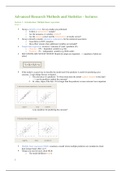
If the model is a good way to describe the model and if the predictor is useful for predicting your
outcome. 2 main things that are evaluated:
1. The relevance of a predictor: To what extent does the model explain variation in the data?
—> can the predictor explain the outcome?
2. B- value, slope of the line: if it is larger than the predictor is more relevant: how important
is my predictor for predicting the outcome?
Multiple linair regression (MLR): examines a model where multiple predictors are included to check
their unique linear effect on Y
Things you need to know about MLR:
o The model (different trends)
1
, o The types of variables in MLR
o MLR and hierarchical MLR
Hypotheses
Output
Model fit: R2, adjusted R2, R2-change
Regression coefficients: B and Beta (standardized B)
o Exploratory MLR (stepwise) vs. Confirmatory MLR (forced entry)
o Model assumptions important to MLR
The model
Outcome variable: y, because it is placed on the y-axis when you plot things
Intercept:
Slope:
Residual: some error in the prediction
Observed outcome: prediction based on the model and some error in prediction
Y hat: prediction!!! (Y met dakje) —> will probably not be exactly the observed outcome —> this is
called the statistical model, MLR e.g.
Subscript i: notes that each individual can have a different score
Terms without subscript i’s: parameters, stay the same over the different individual scores
Additive linear model: multiple predictors, assume that the predictions are additive! (+, +) —> different
then e.g. Correlation models (interaction effects)
Main effect: x1, x2, look at a model where they are both added in the model
Types of variables
Formal distinctions in 4 measurements levels, logical order (lowest to highest level of complexity)
o Nominal
o Ordinal
o Interval
o Ratio
For choice of analysis we usually distinguish:
o Nominal + ordinal: categorical or qualitative
o Interval + ratio: continuous or quantitative or numerical —> allowed to make computations
with this variable
Rule 1 in MLR: the outcome is always continuous AND continuous predictors!!!
o Is created for the situation where all the variables are continuous
o One exception: if you want to include a categorical predictor, that’s possible, but you have to
use dummy variables
Dummy coding in MLR models: e.g., is gender a predictor of grade?
o Gender: create a dummy variable, e.g. 0 = male, 1 = female (ALWAYS a 1/0 variable!!)
2
, More predictors? Create more dummy variables!
o E.g., one to denote red(1) or not red (0)
o One to denote blue (1) or not blue (0)
o One to denote green (1) or not green (0)
o If all the dummy’s are 0 you will know it is 0 —> reference group (group with 0’s on all
dummy’s)
Predicted score on the outcome is a certain intercept —> average on y for the reference group (0’s on
all dummy’s so 3 terms disappear)
Hierarchical MLR
Output 1
For each model must be HA: R2(-change) > 0
o R-squared change > 0 means that the additional predictors improve the model
For each predictor x within each model: HA: B1 is not 0 —> unique effect of x within this model
Output 1: you can see 2 models. Always read the titles, columns and footnotes!
o In the model summary you can see R, R squared, adjusted R squared
R-squared: proportion of variance in the outcome variable explained by the model —> computed for
your sample
o Inferential statistics: using a sample to say something about the population
o Not a very good estimate for the population R-squared… Always a little bit too optimistic/high
More predictors, more optimistic! (Bias)
R: square root of R-squared. This is called multiple correlation coefficient: correlation between
observed Y’s en predicted Y’s (capital R to denote that it’s a multiple correlation and not bivariate!!!)
Adjust R-squared: somewhat smaller than unadjusted.
o Corrected for the bias of the sample, then you get the adjusted R-squared
o Says something about your guess about the population variance!
R-squared change says something about the difference between the two models. So R-squared change
0.127 for model 2 says something about the difference between model 2 and model 1 (significant
improvement)
Model summary: says something about the addition of new variables to the model, how do they
compare to each other? Is it a significant addition?
3
Lecture 1 – Introduction: Multiple linear regression
Week 1
Always critically review the way studies are performed
o Is there a representative sample?
o Are the measures or variables reliable?
o Are the analysis correct and the interpretation of results correct?
Always critically consider alternative explanations for the statistical association
o Association is NOT causation
o Does effect remain when additional variables are included?
Simple linair regression: involves 1 outcome (Y) and 1 predictor (X)
o Outcome = DV = dependent variable (e.g. IQ)
o Predictor = IV = independent variable (e.g. Birth order)
EQUATIONS ARE NEVER TESTED! Models & output are important —> equations of plots are
tested
If the model is a good way to describe the model and if the predictor is useful for predicting your
outcome. 2 main things that are evaluated:
1. The relevance of a predictor: To what extent does the model explain variation in the data?
—> can the predictor explain the outcome?
2. B- value, slope of the line: if it is larger than the predictor is more relevant: how important
is my predictor for predicting the outcome?
Multiple linair regression (MLR): examines a model where multiple predictors are included to check
their unique linear effect on Y
Things you need to know about MLR:
o The model (different trends)
1
, o The types of variables in MLR
o MLR and hierarchical MLR
Hypotheses
Output
Model fit: R2, adjusted R2, R2-change
Regression coefficients: B and Beta (standardized B)
o Exploratory MLR (stepwise) vs. Confirmatory MLR (forced entry)
o Model assumptions important to MLR
The model
Outcome variable: y, because it is placed on the y-axis when you plot things
Intercept:
Slope:
Residual: some error in the prediction
Observed outcome: prediction based on the model and some error in prediction
Y hat: prediction!!! (Y met dakje) —> will probably not be exactly the observed outcome —> this is
called the statistical model, MLR e.g.
Subscript i: notes that each individual can have a different score
Terms without subscript i’s: parameters, stay the same over the different individual scores
Additive linear model: multiple predictors, assume that the predictions are additive! (+, +) —> different
then e.g. Correlation models (interaction effects)
Main effect: x1, x2, look at a model where they are both added in the model
Types of variables
Formal distinctions in 4 measurements levels, logical order (lowest to highest level of complexity)
o Nominal
o Ordinal
o Interval
o Ratio
For choice of analysis we usually distinguish:
o Nominal + ordinal: categorical or qualitative
o Interval + ratio: continuous or quantitative or numerical —> allowed to make computations
with this variable
Rule 1 in MLR: the outcome is always continuous AND continuous predictors!!!
o Is created for the situation where all the variables are continuous
o One exception: if you want to include a categorical predictor, that’s possible, but you have to
use dummy variables
Dummy coding in MLR models: e.g., is gender a predictor of grade?
o Gender: create a dummy variable, e.g. 0 = male, 1 = female (ALWAYS a 1/0 variable!!)
2
, More predictors? Create more dummy variables!
o E.g., one to denote red(1) or not red (0)
o One to denote blue (1) or not blue (0)
o One to denote green (1) or not green (0)
o If all the dummy’s are 0 you will know it is 0 —> reference group (group with 0’s on all
dummy’s)
Predicted score on the outcome is a certain intercept —> average on y for the reference group (0’s on
all dummy’s so 3 terms disappear)
Hierarchical MLR
Output 1
For each model must be HA: R2(-change) > 0
o R-squared change > 0 means that the additional predictors improve the model
For each predictor x within each model: HA: B1 is not 0 —> unique effect of x within this model
Output 1: you can see 2 models. Always read the titles, columns and footnotes!
o In the model summary you can see R, R squared, adjusted R squared
R-squared: proportion of variance in the outcome variable explained by the model —> computed for
your sample
o Inferential statistics: using a sample to say something about the population
o Not a very good estimate for the population R-squared… Always a little bit too optimistic/high
More predictors, more optimistic! (Bias)
R: square root of R-squared. This is called multiple correlation coefficient: correlation between
observed Y’s en predicted Y’s (capital R to denote that it’s a multiple correlation and not bivariate!!!)
Adjust R-squared: somewhat smaller than unadjusted.
o Corrected for the bias of the sample, then you get the adjusted R-squared
o Says something about your guess about the population variance!
R-squared change says something about the difference between the two models. So R-squared change
0.127 for model 2 says something about the difference between model 2 and model 1 (significant
improvement)
Model summary: says something about the addition of new variables to the model, how do they
compare to each other? Is it a significant addition?
3