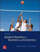
A complete (!) summary of the book Applied Statistics in Business and Economics for the first year course Business Statistics of International Business Administration (IBA).
An observation is a single member of a collection of items we want to study.
A variable is a characteristic of the subject or individual.
The data set consists of all the values of all the variables for all the observations we have
chosen to observe. Each column is a variable, each row is an observation.
A data set may contain a mixture of data types. Two broad categories are categorial data
and numerical data.
Categorial data (also qualitative data, described by labels) have values that are described by
words rather than numbers, it cannot be described with numbers. Coding is when the
categorial variables are represented by numbers.
Numerical data (also quantitative data, meaningful numbers) arises from some kind of
mathematical operation, such as measurement or counting. Numerical data can be of two
types: discrete and continuous.
Discrete means a variable with a countable number of distinct values.
Continuous is a numerical variable that can have any value within an interval.
§2.2 Level of measurement
Measurement for data is divided in 4 levels: nominal, ordinal, interval and ratio.
Nominal data merely identify a category. Nominal is the same as categorial data. Nominal
data is usually coded numerically. Only counting is allowed.
Ordinal data can be used to rank data values. Counting and order statistics are allowed.
Interval data can be used to rank data and has meaningful intervals between scale points.
Sums and differences are allowed.
Ratio data have all the properties of the other three data types, but in addition possesses a
meaningful zero point. What matters is that the 0 is an absolute reference point. The 0 has
to be meaningful, the variable has to be “nothing”, it can’t exist at 0. “If you have 2 of
something, you have to have 2 times the amount of 1 of something”. Any math operations
are allowed.
§3.1 Stem-and-leaf displays and dot plots
Methods to summarize data can be visual (charts and graphs) or numerical (statistics or
tables). Data can be discussed in terms of 3 characteristics: center, variability and shape.
,When you use random sampling, you must allow for sampling error. That is, the possibility
that the used sample is not representative of the total population.
Descriptive measures derived from a sample (n items) are statistics, while for a population
(N items or infinite) they are parameters. For a sample of numerical data, we are interested
in center (where are the data values concentrated?), variability (How spread out are the
data values?) and shape (Are the data values distributed symmetrically?).
§4.2 Measures of center
When we speak of center, we are trying to describe the middle or typical values of a
distribution.
The most familiar statistical measure of center is the mean. It is the sum of the data values
divided by the number of data items. For population µ, for a sample x .
n
1
Sample Mean : x= ∑ X i
n i=1
n
1
Population Mean :µ= ∑X
N i=1 i
The median is the 50th percentile or midpoint of the sorted sample data set x 1 , x 2 , … , x n.
The mode is the most frequently occurring data value.
In symmetric data, the mean and the median are the same. When the data are skewed
right, the mean exceeds the median. When the data are skewed left, the mean is below the
median.
The geometric mean G is a multiplicative average, obtained by multiplying the data values
and then taking the nth root of the product. N is the number of data measures. This is a
measure of central tendency used when all the data values are positive.
G= √n x 1 x 2 … xn
xn
The average growth rate for a time series GR is GR=
measures.
√
n−1
x1
−1. N is the number of data
,The midrange is the point halfway between the lowest and highest values of X. It is useful
when you have Xmin and Xmax.
Xmin+ Xmax
Midrange=
2
The trimmed mean is the normal mean, except that the highest and lowest k percent of the
observations in the sorted data are removed. The trimmed mean mitigates the effects of
extreme high values on either end.
§4.3 Measures of variability
The range is the difference between the largest and smallest observations:
Range = Xmax – Xmin.
The variance is defined as the sum of squared deviations from the mean divided by the
population size:
N
∑ ( xi −µ )2
Population variance :σ 2= i =1
N
N
∑ ( xi −x )2
i=1
Sample variance=
n−1
The standard deviation is a number that helps understanding how individual values in a
data set vary from the mean. Because the square root is taken, its units of measurement are
the same as X.
n
Standard deviation population :σ =
n
√ ∑ ( xi −µ )2
i =1
N
∈short : √ population variance
Standard deviation sample : σ=
√ ∑ ( x i−x )2
i=1
n−1
,∈short : √ sample variance
The coefficient of variation CV is used to compere dispersion in data sets with dissimilar
units of measure. It is expressed as a percent of the mean.
s
CV =100 ∙
x
§4.5 Percentiles, quartiles, and box plots
, When the sample is large, we can meaningfully divide data into 100 groups (percentiles).
Percentiles generally have to be interpolated between two data values.
Alternatively, we can divide the data into 10 groups (deciles), 5 groups (quintiles), or 4
groups (quartiles). The quartiles (denoted Q1, Q2, Q3) are scale points that divide the
sorted data into four groups of approximately equal size, that is, the 25 th, 50th and 75th
percentiles, respectively. The second quartile Q2 is the median.
The interquartile range (IQR) Q3 – Q1 measures the degree of spread in the data (the middle
50%).
A useful tool of exploratory data analysis is the box plot (also called box-and-whisker plot)
based on the five-number summary: Xmin, Q1, Q2, Q2, Xmax.
A box plot shows center (position of the median Q2), variability (width of the “box” defined
by Q1 and Q3 and the range between Xmin and Xmax) and shape (skewness if the whiskers
are of unequal length and/or if the median is not in the center of the box).
§4.6 Correlation and covariance
The sample correlation coefficient describes the degree of linearity between paired
observations on two quantitative variables X and Y. The data set consists of n pairs (x,y) that
are usually displayed on a scatter plot. The correlation coefficient R measures only linear
relationships. R(x,y) = 0 doesn’t mean that x and y are independent.
n
∑ (xi −x)( y i− y) SXY
i=1
Sample correlation coefficient : r= ,∈short r=
n n SX ∙ SY
√∑
i =1
( xi −x )
σXY
2
√∑
i=1
2
( y i− y )
Population correlation coefficient ∈short r=
σX ∙ σY
Its range is -1 ≤ r ≤ +1. When r is near 0, there is little or no linear relationship between X
and Y. An r value near +1 indicates a strong positive relationship, while a value near -1
indicates a strong negative relationship.
The covariance of two random variables X and Y is denoted as Cov(X,Y) or σxy . It is the
degree to which the values of X and Y change together.
N
∑ ( x i−µ X )( y i−µY )
i=1
Covariance for a population :σxy=
N
N
∑ (xi −x)( y i− y)
Covariance for a sample : sxy= i=1
n−1
§4.8 Skewness and Kurtosis
The benefits of buying summaries with Stuvia:
Guaranteed quality through customer reviews
Stuvia customers have reviewed more than 700,000 summaries. This how you know that you are buying the best documents.
Quick and easy check-out
You can quickly pay through credit card or Stuvia-credit for the summaries. There is no membership needed.
Focus on what matters
Your fellow students write the study notes themselves, which is why the documents are always reliable and up-to-date. This ensures you quickly get to the core!
Frequently asked questions
What do I get when I buy this document?
You get a PDF, available immediately after your purchase. The purchased document is accessible anytime, anywhere and indefinitely through your profile.
Satisfaction guarantee: how does it work?
Our satisfaction guarantee ensures that you always find a study document that suits you well. You fill out a form, and our customer service team takes care of the rest.
Who am I buying these notes from?
Stuvia is a marketplace, so you are not buying this document from us, but from seller TiborB. Stuvia facilitates payment to the seller.
Will I be stuck with a subscription?
No, you only buy these notes for $7.43. You're not tied to anything after your purchase.