Analytics for Business and Governance
Week 1 – Introduction and Foundations
Introduction
Course consists of 7 weeks
• 1 Lecture, mainly short clips combined with slides (no lecture on Tuesday)
• 1 Question time via live Zoom sessions – including use of Excel via own laptop (on Thursdays).
• Three case studies/assignments (20% grade, combined).
• Final exam: April 7 (80% grade, OPEN-BOOK).
• Resit counts for 100%.
Assignments are in EXCEL, but the exam is going to be theoretical and should be calculated by HAND.
Open-book exam: all materials should be physical (no online book, printed summaries/slides).
• Excel output question
• 2 Modeling questions: not sure how to upload that answer.
Theory: Chapter 1 (and Chapter 2 as self-study)
Chapter 1 – Introduction to Business Analytics
Business Analytics is the use of:
• Data
• Information technology
• Statistical analysis
• Quantitative methods
• Mathematical or computer-based models
To help managers gain improved insight about their business operations and make better, fact-based decisions.
Examples of Applications
• Pricing: setting pricing for consumer and industrial goods, government contracts and maintenance contracts.
• Customer segmentation: identifying and targeting key customer groups in retail, insurance, and credit card industries.
• Merchandising: determining brands to buy, quantities, and allocations.
• Location: finding the best location for bank branches and ATMs, or where to service industrial equipment.
• Social media: understand trends and customer perceptions; assist marketing managers and product designers.
Impacts and Challenges
Benefits: reduced costs, better risk management, faster decisions, better productivity and enhanced bottom-line performance
such as profitability and customer satisfaction.
Challenges: lack of understanding how to use analytics, competing business priorities, insufficient analytical skills, difficulty in
getting good data and sharing information and not understanding the benefits vs. perceived costs of analytics studies.
Scope of Business Analytics
• Descriptive: the use of data to understand the past and current business
performance and make informed decisions.
How much did we sell in each region? What was our inventory costs last quarter?
• Predictive: predict the future using quantitative methods, e.g. by examining
historical data, detecting patterns or relationships in these data and then
extrapolating these relationships forward in time.
How much we expect to pay for fuel costs next year?
• Prescriptive: identify the best alternatives to minimize or maximize some objective.
What is the best way of shipping goods from our factories to minimize labor costs?
Example 1.1: Retail Markdown Decisions (big data)
• Most department stores clear seasonal inventory by reducing prices.
• Key question: when to reduce the price and by how much to maximize revenue?
• Potential applications of analytics:
o Descriptive analytics: examine historical data for similar products (prices, units sold).
o Predictive analytics: predict sales based on price.
o Prescriptive analytics: find the best sets of pricing and advertising to maximize sales revenue
Big Data
Refers to massive amounts of business data from a wide variety of sources, much of which is available in real time, and much of
which is uncertain or unpredictable (IBM: volume, variety, velocity and veracity).
• Metric: unit of measurement that provides a way to objectively quantify performance, e.g. net profit.
o Discrete: numbers
o Continuous: scale of measurement
• Measurement: the act of obtaining data associated with a metric.
• Measures: numerical associated with a metric.
Little data – big calculations: we would like to visit 25 addresses, what is the shortest route? → an efficient algorithm takes few
seconds to compute!
Models in Business Analytics
Model: an abstraction or representation of a real system, idea or object.
• Captures the most important features
• Can be written or verbal description, a visual representation, a mathematical formula, or a spreadsheet.
1
,Example 1.4: Three Forms of a Model (new product sales over time)
The sales of a new product, such as a first-generation iPad or 3D television, often follow a common pattern.
1. Verbal description: the rate of sales starts small as early adopters begin to
evaluate a new product and then begins to grow at an increasing rate over time as
positive customer feedback spreads. Eventually, the market begins to become
saturated and the rate of sales begins to decrease.
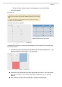
2. Visual model: a sketch of sales as an S-shaped curve over time →
3. Mathematical model: S = aebect, where S is sales, t is time, e is the base of natural
logarithms, and a, b, and c are constants (Gompertz curve).
This is what analytics professionals do.
Decision Models
A logical or mathematical representation of a problem or business situation that can be used to understand, analyze, or facilitate
making a decision.
It is important to keep on mind: all models are only representations of the real world and as such can’t capture every nuance
that the decision maker faces in reality.
Inputs of the model:
• Data: assumed to be constant for purposes of the model (e.g., machine capacities, distances etc.)
• Uncontrollable variables: which are quantities that can change but cannot be directly controlled by the decision
maker (always random, e.g., customer demand, inflation rates, weather conditions).
• Decision variables: are controllable and can be selected at the discretion of the decision maker (e.g., production
quantities, staffing levels, the location of a warehouse).
Outputs of the model:
• Measures of performance or behavior (e.g., profit, mean waiting time,
total CO2 emissions).
Example 1.6: Building a Mathematical Model
• Total Cost (TC) = Fixed Cost (F) + Variable Cost (V)
• V = Unit V * Quantity produced (Q)
• TC = F + V * Q
Example 1.7: A Break-Even Decision Model
We would like to find the demand level Q, above which it becomes more economical to manufacture in house instead of
outsourcing.
TC(manufacturing) = $50,000 + $125*Q
TC(outsourcing) = $175*Q
Break-even point: TC(manufacturing) = TC(outsourcing) NAAST ELKAAR ZETTEN EN WEGSTREPEN
• Q = 1,000
• Q = F / (C-V)
Example 1.8: A Sales-Promotion Decision Model
In the grocery industry, managers typically need to know how best to use pricing, coupons, and advertising strategies to
influence sales. Grocers often study the relationship of sales volume to these strategies by conducting controlled experiments to
identify the relationship between them and sales volumes. That is, they implement different combinations of pricing, coupons,
and advertising, observe the sales that result, and use analytics to develop a predictive model of sales as a function of
these decision strategies. We can use such a model to evaluate different strategies and help to choose the best to maximize
sales or profitability.
• Example Model: if the price is $6.99, no coupons are offered and no advertising is done (the experiment corresponding to
week 1), the model estimates sales as:
• Sales = 500 – 0.05(price) + 30(coupons) + 0.08(advertising) + 0.25(price)(advertising) predicting effects of input
(estimated from existing data
• 500 – 0.05*$6.99 + 30*0 + 0.08*0 + 0.25*$6.99*0 = 499.65 units ~ 500 units.
Model Assumptions
Assumptions are made to:
1. Simplify a model and make it more tractable; that is, able to be easily analyzed or solved.
2. Better characterize historical data or past observations.
The task of the modeler is to select or build an appropriate model that best represents the behavior of the real situation.
Example 1.9: A linear Demand Prediction model: D = a – bP.
As price increases, demand falls.
Example 1.10: A Nonlinear Demand Prediction Model: D = cP-d
For example: D = 20000P-0.0111382, if you plot you will see that the two curves are very similar. From
the modeler perspective, we prefer the linear model as they are easier to work with in general.
Uncertainty and Risk
Uncertainty: is imperfect knowledge of what will happen in the future.
Risk: is associated with the consequences of what actually happens.
The stock price of Apple tomorrow is uncertain. Uncertainty has no impact on me if I don’t own Apple stock. If I do, I bear the
risk of losing money. Risk is an outcome of uncertainty.
We can’t eliminate uncertainty, but we can do something about our risk exposure.
Prescriptive Decision Models
2
, Help decision makers identify the best solution.
Optimization: finding values of decision variables that minimize (or maximize) something such as cost (or profit).
• Objective function: the equation that minimizes (or maximizes) the quantity of interest
• Constraints: limitations or restrictions.
• Optimal solution: values of the decision variables at the minimum (or maximum) point.
Example 1.11: A Prescriptive Pricing Model
• A firm wishes to determine the best pricing for one of its products in order to maximize revenue.
• Analysts determined the following model:
• Sales = -2.9485(price) + 3240.9
• Total revenue = (price)(sales) = price*(-2.9485*price+3240.9) = -2.9485*price2+3240.9*price
Identify the price that maximizes total revenue, subject to any constraints that might exist. (who knows how this can be done fe)
Types of Prescriptive Models
Deterministic model: all model input information is known with certainty.
Stochastic model: some model input information is uncertain.
• F.e.: suppose that customer demand is an important element of some model. We can make the assumption that the
demand Is known with certainty; say, 5000 units per month (deterministic). On the other hand, suppose we have evidence
to indicate that demand is uncertain, with an average value of 5000 units per month, but which typically varies between
3200 and 6800 units (stochastic).
Problem Solving with Analytics
1. Recognizing a problem
2. Defining the problem
3. Structuring the problem
4. Analyzing the problem
5. Interpreting results and making a decision
6. Implementing the solution
Chapter 5 – Probability Distributions and Data Modeling
Basic Concepts of Probability
Probability: is the likelihood that an outcome occurs. Expressed as values between 0 and 1. Ex: if fair, then 1/6
Experiment: is the process that results in an outcome. Ex: roll a die
Outcome: (of an experiment) is a result that we observe. Ex: what # came out
Sample space: is the collection of all possible outcomes of an experiment. Ex: {1,2…6}
Definitions of Probability
Probabilities may be defined from one of three perspectives:
• Classical definition: probabilities can be deduced from theoretical arguments.
• Relative frequency definition: probabilities are based on empirical data.
• Subjective definition: probabilities are based on judgment and experience. Ex: what do you think is the probability etc.
Ex: roll 2 dice.
• Possible outcomes: {(1,1)(1,2)…(6,6)} 36 outcomes and they are equally likely (1/36).
• (i,j) and, x = i + j (dice sum)
• Smallest number is going to be 2 (1+1) and largest number is going to be 12 (6+6)
• X{2,….12}
• P(X=2) = there is only one outcome that gives 2 so: 1/36 probability
• P(X=3) = there are 2 options that give X = 3 (2 + 1 and 1 + 2) so: 2/36 probability
• P(X=7) options: (1,6), (2,5), (3,4), (4,3), (5,2), (6,1) all give X=7, so there are 6 options: 6/36
probability
Example: Relative Frequency Definition of Probability
• Use relative frequencies as probabilities
• Probability a computer is repaired in 10 days = 0.076
• Data from Computer Repair Times (table)
• If we sum all the numbers under Frequency, we will get the total number of instances.
• Divide 19/total number of instances you will get: Relative Frequency.
• We are given that the Relative Frequency is 0.076 and Frequency is 19 so:
• 0.076 = 19 / (?), to calculate (?) = .076 = 250 total number of instances/observations in total!
• Also interested in Cumulative Percentage: calculated by the CumulativePercentaget-1 + RelativeFrequencyt
• Cumulative percentage: probability that it will be
repaired in less than or equal to 10 days = 0.212
(13.6% equals 0.136 + 0.076 = 0.212).
Probability Rules and Formulas
• Label the n outcomes in a sample space as O1,
O2,…,On, where Oj represents the jth outcome in the
sample space. Let P(Oj) be the probability associated
with the outcome Oj.
• The probability associated with any outcome must
be between 0 and 1.
o 0 ≤ 𝑃(𝑂𝑗 ) ≤ 1 for each outcome Ojj
• The sum of the probabilities over all possible outcomes must be equal to 1.
3


