Laplace Transform
CHAPTER 4
LAPLACE TRANSFORM
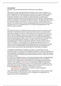
Concept Mapping
function
Unit step function
- Linearity
theorem - First shift theorem
- First shift Unit impulse function
- multiplying with r' - ofix up' function of s by
- dividing by I (D multiplying/ dividing Periodic function
by appropriate constant
(ii) completing square
(iii) partial fraction
- transform of integral
- Convolution theorem
Solve first-order, second-order or system of linear DE
Objective
At the end of this chapter, students should be able to:
(a) Find the Laplace transform by definition or applying the properties,
such as linearity, first shift theorem, multiplying a function with t",
dividing a function by t.
(b) Find inverse Laplace transform by applying properties or theorem such
as linearity, first shift theorem, 'fix up' a function by multiplying and
dividing by a appropriate constant, completing square, partial fraction
decomposition, transform of integral, and convolution theorem.
(c) Solve the first-order, second-order or system of linear differential
equations with constant coefficients by Laplace transform.
(d) Find the Laplace transform of non-continuous functions such as unit
step function, unit impulse function and periodic function.
(e) Solve the nonhomogeneous first-order, second-order or system of
linear differential equations for non-continuous function by Laplace.
(D Apply the Laplace transform in electrical circuit systems.
Key Term (English - Bahasa Melayu)
Convolution theorem Teorem Konvolusi
First shift theorem Teorem anjakan pertama
Inverse Laplace transform Jelmaan Laplace songsang
Laplace ffansform Jelmaan Laplace
Linearity Kelinearan
Periodic function Fungsi berkala
Second shift theorem Teorem anjakan kedua
Transform of integral Jelmaan kamiran
Unit impulse function Fungsi impuls unit
Unit step function Fungsi langkah unit
95
, Laplace Transform
In chapter 1 to 3, the ordinary differential equations considered are in
the form ,f , cy = f (x),where f(x) isthe continuous function.
dffu+b**
However, the discontinuous funetions are not uncommon for physical system.
For example, for the mathematical model of electrical circuit system, i.e.
L+*R+**=E(r), the impressed voltage, E(t), ona circuit could be
dt' dt C
piecewise, impulsive or periodic function. Solving the ordinary differential
equations of the circuit of this case is difficult using the method of solutions in
chapter 1 and 2. Thus, the Laplace transform studied in this chapter is an
invaluable tool that simplifies solving problems such as these.
4.1.1 Definition of Laplace Transform
Suppose f (t) is a function which is defined in [0,oo), then the integral
,-" f (t) dt = 4.f @]
[*
is said to be the Laplace transform of the funetion f(t), provided the
integral converges.
From the definition of Laplace transform, notice that the interval r is
0< t < oo . It means that the Laplace transform is only defined in the non-
negative r-axis! since is an improper integral, it is solved by
J-e-"f(t)dt
applying the limit concept as below.
li u-" f (,) d, =
ly f e-"'f (t) dt ,
provided the limit when 7 approaches m exist, or in other words, the integral
converges. The result is a function of s. The notation <if Laplace transform is
given as below.
tUtt>j= ff e-" f (t) dt = F(s)
96
, Laplace Transform
The symbol 'I' above is an operator. Generally, we use a lowercase
letter to denote the function being transformed and the corresponding capital
letter to denote its Laplace transform. For example,
r{g(r)}= G(s), c{y1t1}= Yg), cfQ)}= /(s) etc.
Examole 4.1
py applying the definition, find the Laplace transforrn of
(a) f(t)=a, (b) f(t)=t,
(c) .f (t) = e'' , (d) .f (t) = sinal, where a is constant.
Solution:
(a) t{a}= ffr-"o at =olr*ffe-" dt
Ls-,r*lrrl
r+o[s ,-,,1' =rt.[-
=or*f-l
Jo r+ols s _l
= orm[10__r-,rrf
r+-[^s .J=! s
Note: lim e-'r = e* x 0
T+o
(b) Lt\ = ff u-", d, =
|ry f, e-" t dt by using tabular integration
t e-n
l-
rm[-
= r_+.1 -
.s s, J
e-"1' f r+ e-"
i\a
o
= m[-:'
-sr
- L'-sr-(-' -i ,')]
Ig[-:' -sr L"'sr.i]
= - =
i
(c) ,?'\= f,e-"so' d, =l*f e-<'-")t dt
tm[-
= r_+ol J-"-r,-r,)'
(s _ a) I o
| ,-r'-o)r + | e,l =-L
m[-(s-a)
= r-+ol
'
s-a t-o )
101 r{sinar}= }g ff ,-" sinat dt By integration by
e-" sinar u =sinat dv = e-" dt
11*[-
= r-+ol-
s - Jf-9r-* "rro,
drl' du=acosat u=*
Jo
" By ludv =uu- Iudu
_ e* sino
+o+ I ll e_,, cosq at
s sJo
By integration by parts,
97
, Laplace Transform
=:[[=P], ; ri,-"",,*n) u= cosat dv = e-"' dt
du=-asinat r=*
=
i[o (+) -1ff,-" sinat dtf By fudv =uu- lndu
=3-i f "" sinat dt =i-|r{sinar}
Rearranging, we have
inat\=g
[,.5),0
" *:::
. :::::l .? ...n . . ....rry eues,ion,, Exercise 4A
By using the results of part (a), Example 4.1, we can generalize the
,{1} i ,' . In the simitar case, by using the results
following: r{:}= 1,
,s 14)= s = 4s
of part (c), Example 4.1, we can generalize the following:
U s- j 2s-l' -' t s-(-2) s+2-
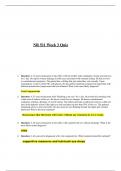
The following table shows some common Laplace transform which
can be obtained by using the definition of Laplaoe transform.
Table 4.1 : The table of Laplace transform
a a
sinat
s 7;7
eo' 1 J
cosat
s-a s'+a'
tn when n! a
n=0,1,2,... F sinhar --;------;
s'-a'
s
cosh af
7:V
From Table 4.1, we notice that the function F exists in the s domain
rather than the r domain of the functionl Anyway, the variables s is not a time
or length or any other physical quantity. Normally, we regard domain I as time
domain and domain s as frequency domain. Besides, the Laplace transform
often produces a function whose character iqentirely different from that of the
input function. For example, the exponent function, e'' and the trigonometric
functions, says sin at have rational functions for their Laplace transform.
98
CHAPTER 4
LAPLACE TRANSFORM
Concept Mapping
function
Unit step function
- Linearity
theorem - First shift theorem
- First shift Unit impulse function
- multiplying with r' - ofix up' function of s by
- dividing by I (D multiplying/ dividing Periodic function
by appropriate constant
(ii) completing square
(iii) partial fraction
- transform of integral
- Convolution theorem
Solve first-order, second-order or system of linear DE
Objective
At the end of this chapter, students should be able to:
(a) Find the Laplace transform by definition or applying the properties,
such as linearity, first shift theorem, multiplying a function with t",
dividing a function by t.
(b) Find inverse Laplace transform by applying properties or theorem such
as linearity, first shift theorem, 'fix up' a function by multiplying and
dividing by a appropriate constant, completing square, partial fraction
decomposition, transform of integral, and convolution theorem.
(c) Solve the first-order, second-order or system of linear differential
equations with constant coefficients by Laplace transform.
(d) Find the Laplace transform of non-continuous functions such as unit
step function, unit impulse function and periodic function.
(e) Solve the nonhomogeneous first-order, second-order or system of
linear differential equations for non-continuous function by Laplace.
(D Apply the Laplace transform in electrical circuit systems.
Key Term (English - Bahasa Melayu)
Convolution theorem Teorem Konvolusi
First shift theorem Teorem anjakan pertama
Inverse Laplace transform Jelmaan Laplace songsang
Laplace ffansform Jelmaan Laplace
Linearity Kelinearan
Periodic function Fungsi berkala
Second shift theorem Teorem anjakan kedua
Transform of integral Jelmaan kamiran
Unit impulse function Fungsi impuls unit
Unit step function Fungsi langkah unit
95
, Laplace Transform
In chapter 1 to 3, the ordinary differential equations considered are in
the form ,f , cy = f (x),where f(x) isthe continuous function.
dffu+b**
However, the discontinuous funetions are not uncommon for physical system.
For example, for the mathematical model of electrical circuit system, i.e.
L+*R+**=E(r), the impressed voltage, E(t), ona circuit could be
dt' dt C
piecewise, impulsive or periodic function. Solving the ordinary differential
equations of the circuit of this case is difficult using the method of solutions in
chapter 1 and 2. Thus, the Laplace transform studied in this chapter is an
invaluable tool that simplifies solving problems such as these.
4.1.1 Definition of Laplace Transform
Suppose f (t) is a function which is defined in [0,oo), then the integral
,-" f (t) dt = 4.f @]
[*
is said to be the Laplace transform of the funetion f(t), provided the
integral converges.
From the definition of Laplace transform, notice that the interval r is
0< t < oo . It means that the Laplace transform is only defined in the non-
negative r-axis! since is an improper integral, it is solved by
J-e-"f(t)dt
applying the limit concept as below.
li u-" f (,) d, =
ly f e-"'f (t) dt ,
provided the limit when 7 approaches m exist, or in other words, the integral
converges. The result is a function of s. The notation <if Laplace transform is
given as below.
tUtt>j= ff e-" f (t) dt = F(s)
96
, Laplace Transform
The symbol 'I' above is an operator. Generally, we use a lowercase
letter to denote the function being transformed and the corresponding capital
letter to denote its Laplace transform. For example,
r{g(r)}= G(s), c{y1t1}= Yg), cfQ)}= /(s) etc.
Examole 4.1
py applying the definition, find the Laplace transforrn of
(a) f(t)=a, (b) f(t)=t,
(c) .f (t) = e'' , (d) .f (t) = sinal, where a is constant.
Solution:
(a) t{a}= ffr-"o at =olr*ffe-" dt
Ls-,r*lrrl
r+o[s ,-,,1' =rt.[-
=or*f-l
Jo r+ols s _l
= orm[10__r-,rrf
r+-[^s .J=! s
Note: lim e-'r = e* x 0
T+o
(b) Lt\ = ff u-", d, =
|ry f, e-" t dt by using tabular integration
t e-n
l-
rm[-
= r_+.1 -
.s s, J
e-"1' f r+ e-"
i\a
o
= m[-:'
-sr
- L'-sr-(-' -i ,')]
Ig[-:' -sr L"'sr.i]
= - =
i
(c) ,?'\= f,e-"so' d, =l*f e-<'-")t dt
tm[-
= r_+ol J-"-r,-r,)'
(s _ a) I o
| ,-r'-o)r + | e,l =-L
m[-(s-a)
= r-+ol
'
s-a t-o )
101 r{sinar}= }g ff ,-" sinat dt By integration by
e-" sinar u =sinat dv = e-" dt
11*[-
= r-+ol-
s - Jf-9r-* "rro,
drl' du=acosat u=*
Jo
" By ludv =uu- Iudu
_ e* sino
+o+ I ll e_,, cosq at
s sJo
By integration by parts,
97
, Laplace Transform
=:[[=P], ; ri,-"",,*n) u= cosat dv = e-"' dt
du=-asinat r=*
=
i[o (+) -1ff,-" sinat dtf By fudv =uu- lndu
=3-i f "" sinat dt =i-|r{sinar}
Rearranging, we have
inat\=g
[,.5),0
" *:::
. :::::l .? ...n . . ....rry eues,ion,, Exercise 4A
By using the results of part (a), Example 4.1, we can generalize the
,{1} i ,' . In the simitar case, by using the results
following: r{:}= 1,
,s 14)= s = 4s
of part (c), Example 4.1, we can generalize the following:
U s- j 2s-l' -' t s-(-2) s+2-
The following table shows some common Laplace transform which
can be obtained by using the definition of Laplaoe transform.
Table 4.1 : The table of Laplace transform
a a
sinat
s 7;7
eo' 1 J
cosat
s-a s'+a'
tn when n! a
n=0,1,2,... F sinhar --;------;
s'-a'
s
cosh af
7:V
From Table 4.1, we notice that the function F exists in the s domain
rather than the r domain of the functionl Anyway, the variables s is not a time
or length or any other physical quantity. Normally, we regard domain I as time
domain and domain s as frequency domain. Besides, the Laplace transform
often produces a function whose character iqentirely different from that of the
input function. For example, the exponent function, e'' and the trigonometric
functions, says sin at have rational functions for their Laplace transform.
98