Methodology, Measurement And Statistics For PM Students (424023B6)
Summary
Summary Applied Statistics I (424023-B-6) - STATISTICS PART
27 views 0 purchase
Course
Methodology, Measurement And Statistics For PM Students (424023B6)
Institution
Tilburg University (UVT)
Book
Applied Statistics I - International Student Edition
This summary covers all subjects seen in the statistics class given by Luc van Baest.
However, it doesn't cover the methodology and SPSS part, so I recommend you take a look at the bundle that includes all three summaries (Statistics + Methodology + SPSS)
Summary for Methods, Measurement and Statistics
Causal Analysis Techniques
All for this textbook (5)
Written for
Tilburg University (UVT)
Premaster Human Resource Studies
Methodology, Measurement And Statistics For PM Students (424023B6)
All documents for this subject (5)
Seller
Follow
cmuyldermans
Content preview
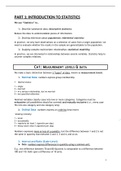
PART 1: INTRODUCTION TO STATISTICS
We use “Statistics” to…
1) Describe/summarize data: descriptive statistics.
Reduce the data to understandable pieces of information.
2) Drawing inferences about populations: inferential statistics
In practice, we only have observations on a selection of cases from a larger population; we
need to evaluate whether the results in the sample are generalizable to the population.
3) Studying complex multivariate relationships: statistical modelling
In practice, we are interested in relationships between several variables. Statistics help to
uncover complex relations.
CH1: MEASUREMENT LEVELS & DATA
We make a basic distinction between 3 “types” of data, known as measurement levels:
1. Nominal Data: numbers express group membership.
Marital status:
1= single
2= married
3= in a serious relationship, but no married
4= not specified otherwise
Nominal variables classify cases into two or more categories. Categories must be
exhaustive (all possibilities should be covered) and mutually exclusive (i.e., every case
fits into one category and one category only).
1= never
2= occasionally
3= regularly (at least 1 cigarette per day).
4= heavy (more than 5 cigarettes per day).
Numbers expresses more or less of a quantity, but the difference between 1 and 2 is not
the same in quantity than between 2 and 3, 3 and 4, and so on.
3. Interval and Ratio (Scale-Level)
Data: numbers express differences in quantity using a common unit.
E.g., the difference between 70 and 80 IQ points is comparable to a difference between
100 and 110. Both span a difference of 10 units.
1
,Within scale data we can distinguish between ratio-level and interval-level:
Ratio-level data have a “natural” zero-point (e.g., length, income). As a result, you can
compare the relative magnitude of things, e.g., you can say that one person is twice as tall
as another person.
Interval level variables don’t have a natural zero point (e.g., “zero temperature is
meaningless), but it is arbitrarily chosen and can differ across scales (e.g., zero Fahrenheit
≠ zero Celsius).
With interval data one can compare intervals, but in contrast to ratio level one cannot
say, for example, that 30 degrees is two times hotter than 15 degrees….
Remarks:
Both interval and ratio-level data are referred to as scale data. The idea is simple:
all variables that are not nominal or ordinal are treated as scale-level variables
(levels used in SPSS)
Measurement level is a property of the measurement values, it is not (!) an
intrinsic property of a variable. E.g., you cannot say that “body height” has interval
level; length can be measured at different levels (think of your gym-class…).
So there is not necessarily a one-to-one relationship between measurement levels
and variables.
Measurement levels determine the kind of statistics and statistical analyses you can
use meaningfully. For example, the mean of a nominal variable is meaningless
(e.g., “the average eye colour). Hence, for the analyses you should always respect
the measurement levels of the variables envisaged.
Many of the commonly used statistical techniques assume scale data. However, for
many variables in the social sciences, it is not evident that data are interval level
(e.g., political interest?) Therefore, it is common practice to simply assume that we
have acquired interval data, without worrying too much if this is really true and this
turns out to be very useful.
CH2: DATA INSPECTION
Every analysis starts with data inspection (“getting to know your data”): its goal is to get
a clear picture of the data by examining one variable at the time (univariate), or pairs of
variables (bivariate):
To accomplish this goal, we use graphs and statistics. Which statistics and graphs are most
appropriate depends on the measurement level (i.e., whether the data are nominal,
ordinal, or scale level)?
2
,In general, we want to know more about…
Central tendency: What are the most common values?
Variability: How large are the differences between the subjects? Are there
extreme values in the sample?
Bivariate Association: for each pair of variables, do they associate/co-vary (i.e.,
do low/large values on one variable go together with low/large values on the other
variable) PART 3
Ordinal/nominal data Scale-level data
CH3: CENTRAL TENDENCY
Mode: the score that is observed most frequently.
Median: the score that separates the higher half of data from the lower half
Example 1: ( N = unequal): 4, 5, 6, 7, 8, 9, 9 => median is 7
Example 2: ( N = equal): 4, 5, 6, 8, 9, 9 => median 7
Mean M =
∑X= ∑ of all scores
N total number of scores
Example:
Sum of deviation to the left is
equal to sum of deviation to the right.
∑ ( xi−M )=0 (3-5) + (4-5) + (8-5) = 0
CH5: VARIABILITY
= not everyone scoring the same
Sum of deviation scores from the mean = 0
Problem! When measuring variability it will always end up being 0; tells us nothing.
Solution Take the square of the sum of deviation scores to make it positive
Σ(X – M)2
Notation Sum of Squares SS = Σ(Xi – M)2
MEASURES OF VARIABILITY
For the exercise above:
VARIANCE: S2 =
∑ ( X −M ) ² = SS Scores (X) = 3,4,8
N−1 df Mean (M) = 5
Deviation scores = (X-M) = -2,
STANDARD VARIANCE (SD): -1, 3
S= √ S ²
MINIMUM/MAXIMUM: lowest/highest observed value S= √ 7=2.65
RANGE: maximum - minimum
NB: The larger the variance
the more different answers
you get.
INTERQUARTILE RANGE (IQR): ranges of scores that
encompass 50% of the middle observations; thus,
excluding the 25% lowest & 25% highest observations
4
The benefits of buying summaries with Stuvia:
Guaranteed quality through customer reviews
Stuvia customers have reviewed more than 700,000 summaries. This how you know that you are buying the best documents.
Quick and easy check-out
You can quickly pay through credit card or Stuvia-credit for the summaries. There is no membership needed.
Focus on what matters
Your fellow students write the study notes themselves, which is why the documents are always reliable and up-to-date. This ensures you quickly get to the core!
Frequently asked questions
What do I get when I buy this document?
You get a PDF, available immediately after your purchase. The purchased document is accessible anytime, anywhere and indefinitely through your profile.
Satisfaction guarantee: how does it work?
Our satisfaction guarantee ensures that you always find a study document that suits you well. You fill out a form, and our customer service team takes care of the rest.
Who am I buying these notes from?
Stuvia is a marketplace, so you are not buying this document from us, but from seller cmuyldermans. Stuvia facilitates payment to the seller.
Will I be stuck with a subscription?
No, you only buy these notes for $7.95. You're not tied to anything after your purchase.