Chapter 10
Dummy Variable Models
In general, the explanatory variables in any regression analysis are assumed to be quantitative in nature. For
example, the variables like temperature, distance, age etc. are quantitative in the sense that they are recorded
on a well-defined scale.
In many applications, the variables can not be defined on a well-defined scale, and they are qualitative in
nature.
For example, the variables like sex (male or female), colour (black, white), nationality, employment status
(employed, unemployed) are defined on a nominal scale. Such variables do not have any natural scale of
measurement. Such variables usually indicate the presence or absence of a “quality” or an attribute like
employed or unemployed, graduate or non-graduate, smokers or non- smokers, yes or no, acceptance or
rejection, so they are defined on a nominal scale. Such variables can be quantified by artificially constructing
the variables that take the values, e.g., 1 and 0 where “1” usually indicates the presence of attribute and “0”
usually indicates the absence of the attribute. For example, “1” indicator that the person is male and “0”
indicates that the person is female. Similarly, “1” may indicate that the person is employed and then “0”
indicates that the person is unemployed.
Such variables classify the data into mutually exclusive categories. These variables are called indicator
variable or dummy variables.
Usually, the indicator variables take on the values 0 and 1 to identify the mutually exclusive classes of the
explanatory variables. For example,
1 if person is male
D
0 if person is female,
1 if person is employed
D
0 if person is unemployed.
Here we use the notation D in place of X to denote the dummy variable. The choice of 1 and 0 to identify
a category is arbitrary. For example, one can also define the dummy variable in the above examples as
Econometrics | Chapter 10 | Dummy Variable Models | Shalabh, IIT Kanpur
1
, 1 if person is female
D
0 if person is male,
1 if person is unemployed
D
0 if person is employed.
It is also not necessary to choose only 1 and 0 to denote the category. In fact, any distinct value of D will
serve the purpose. The choices of 1 and 0 are preferred as they make the calculations simple, help in the easy
interpretation of the values and usually turn out to be a satisfactory choice.
In a given regression model, the qualitative and quantitative can also occur together, i.e., some variables are
qualitative, and others are quantitative.
When all explanatory variables are
- quantitative, then the model is called a regression model,
- qualitative, then the model is called an analysis of variance model and
- quantitative and qualitative both, then the model is called an analysis of covariance model.
Such models can be dealt with within the framework of regression analysis. The usual tools of regression
analysis can be used in the case of dummy variables.
Example:
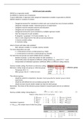
Consider the following model with x1 as quantitative and D2 as an indicator variable
y 0 1 x1 2 D2 , E ( ) 0, Var ( ) 2
0 if an observation belongs to group A
D2
1 if an observation belongs to group B.
The interpretation of the result is essential. We proceed as follows:
If D2 0, then
y 0 1 x1 2 .0
0 1 x1
E ( y / D2 0) 0 1 x1
which is a straight line relationship with intercept 0 and slope 1 .
Econometrics | Chapter 10 | Dummy Variable Models | Shalabh, IIT Kanpur
2
Dummy Variable Models
In general, the explanatory variables in any regression analysis are assumed to be quantitative in nature. For
example, the variables like temperature, distance, age etc. are quantitative in the sense that they are recorded
on a well-defined scale.
In many applications, the variables can not be defined on a well-defined scale, and they are qualitative in
nature.
For example, the variables like sex (male or female), colour (black, white), nationality, employment status
(employed, unemployed) are defined on a nominal scale. Such variables do not have any natural scale of
measurement. Such variables usually indicate the presence or absence of a “quality” or an attribute like
employed or unemployed, graduate or non-graduate, smokers or non- smokers, yes or no, acceptance or
rejection, so they are defined on a nominal scale. Such variables can be quantified by artificially constructing
the variables that take the values, e.g., 1 and 0 where “1” usually indicates the presence of attribute and “0”
usually indicates the absence of the attribute. For example, “1” indicator that the person is male and “0”
indicates that the person is female. Similarly, “1” may indicate that the person is employed and then “0”
indicates that the person is unemployed.
Such variables classify the data into mutually exclusive categories. These variables are called indicator
variable or dummy variables.
Usually, the indicator variables take on the values 0 and 1 to identify the mutually exclusive classes of the
explanatory variables. For example,
1 if person is male
D
0 if person is female,
1 if person is employed
D
0 if person is unemployed.
Here we use the notation D in place of X to denote the dummy variable. The choice of 1 and 0 to identify
a category is arbitrary. For example, one can also define the dummy variable in the above examples as
Econometrics | Chapter 10 | Dummy Variable Models | Shalabh, IIT Kanpur
1
, 1 if person is female
D
0 if person is male,
1 if person is unemployed
D
0 if person is employed.
It is also not necessary to choose only 1 and 0 to denote the category. In fact, any distinct value of D will
serve the purpose. The choices of 1 and 0 are preferred as they make the calculations simple, help in the easy
interpretation of the values and usually turn out to be a satisfactory choice.
In a given regression model, the qualitative and quantitative can also occur together, i.e., some variables are
qualitative, and others are quantitative.
When all explanatory variables are
- quantitative, then the model is called a regression model,
- qualitative, then the model is called an analysis of variance model and
- quantitative and qualitative both, then the model is called an analysis of covariance model.
Such models can be dealt with within the framework of regression analysis. The usual tools of regression
analysis can be used in the case of dummy variables.
Example:
Consider the following model with x1 as quantitative and D2 as an indicator variable
y 0 1 x1 2 D2 , E ( ) 0, Var ( ) 2
0 if an observation belongs to group A
D2
1 if an observation belongs to group B.
The interpretation of the result is essential. We proceed as follows:
If D2 0, then
y 0 1 x1 2 .0
0 1 x1
E ( y / D2 0) 0 1 x1
which is a straight line relationship with intercept 0 and slope 1 .
Econometrics | Chapter 10 | Dummy Variable Models | Shalabh, IIT Kanpur
2