A.1 Assignment 01
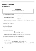
ASSIGNMENT 01
Due date: Wednesday, 20 April 2022
ONLY FOR YEAR MODULE
1. Consider the differential equation
y 0 (x) = −3x 2 y 2 , y(0) = 2,
which has the analytical solution
2
y= .
2x 3 + 1
Apply the modified Euler method to solve the equation up to x = 1 first with steplength h = 0.2 and
then with h = 0.1. At each step make 2 corrections. Also calculate the error at each step.
In your solution include:
(i) description of the algorithms used
(ii) program listing (printout)
(iii) computer results (printout)
(iv) discussion of the results
2. Solve the differential equation
dy
= 3x + 2y + xy, y(0) = −1
dx
by means of the Taylor-series expansion to get the value of y at x = 0.1. Use terms up to x 6 .
3. Consider the system of coupled second-order differential equations
u 00 − (t + 1)uv + v 0 = cos t
v 00 = u 0 + uv
with initial conditions
u(0) = 2, u 0 (0) = 1, v (0) = 3, v 0 (0) = −1.
Use the second-order Runge-Kutta method with h = 0.2 and a = 2/3, b = 1/3, α = β = 3/2, to find
u, u 0 , v and v 0 at t = 0.2.
14
, APM3711/101/0/2022
A.2 Assignment 02
ASSIGNMENT 02
Due date: Monday, 30 May 2022
ONLY FOR YEAR MODULE
1. For the equation
y 0 = y sin (πx) , y(0) = 1,
get starting values by the Runge-Kutta Fehlberg method for x = 0.2, x = 0.4, x = 0.6, and then
advance the solution to x = 1.0 by
(a) Milne’s method,
(b) the Adams-Moulton method.
2. Solve the boundary–value problem
y 00 + x 2 y 0 − 4xy = 2x 3 + 6x 2 − 2, y(0) = 0, y(1) = 2
by using the shooting method. Use the modified Euler method (with only one correction at
each step), and take h = 0.2. Start with an initial slope of y 0 (0) = 1.9 as a first attempt and
y 0 (0) = 2.1 as a second attempt. Then interpolate.
Compare the result with the analytical solution y = x 4 − x 2 + 2x.
3.
(a) The function ex is to be approximated by a fifth-order polynomial over the interval [−1, 1]. Why
is a Chebyshev series a better choice than a Taylor (or Maclaurin) expansion?
(b) Given the power series
f (x) = 1 − x − 2x 3 − 4x 4
and the Chebyshev polynomials
T0 (x) = 1
T1 (x) = x
T2 (x) = 2x 2 − 1
T3 (x) = 4x 3 − 3x
T4 (x) = 8x 4 − 8x 2 + 1,
economize the power series f (x) twice.
(c) Find the Padé approximation R2 (x), with numerator of degree 2 and denominator of degree 1, to
the function f (x) = x 2 + x 3 .
15
, ASSIGNMENT 03
Due date: Monday, 20 June 2022
ONLY FOR YEAR MODULE
1. Solve the boundary–value problem
y 00 + x 2 y 0 − 4xy = 2x 3 + 6x 2 − 2, y (0) = 0, y(1) = 2
by using the shooting method. Use the modified Euler method (with only one correction at each step),
and take h = 0.2. Start with an initial slope of y 0 (0) = 1.9 as a first attempt and y 0 (0) = 2.1 as a
second attempt. Then interpolate.
Compare the result with the analytical solution y = x 4 − x 2 + 2x.
2. (a) Define what is meant by the eigenvalues and eigenvectors of a matrix A.
If the matrix A is
2 0 1
A = −22 −3 10 ,
−12 0 9
(b) find the characteristic polynomial,
(c) find the eigenvalues and eigenvectors.
(d) Start with the approximate eigenvector (1,1,1) and use the power method to estimate the dominant
eigenvalue by iterating 4 times.
(e) Use the power method to find the smallest absolute eigenvalue of A.
(f) Write a program which applies the power method to a given matrix in (d) and (e) above.
3. Consider the following boundary–value problem:
y 00 = 2x 2 y 0 + xy + 2, 1 ≤ x ≤ 4.
Taking h = 1, set up the set of equations required to solve the problem by the finite difference method
in each of the following cases of boundary conditions:
(a) y(1) = −1, y(4) = 4;
(b) y 0 (1) = 2, y 0 (4) = 0;
(c) y 0 (1) = y(1), y 0 (4) = −2y(4).
(Do not solve the equations!).
16
, APM3711/101/0/2022
ASSIGNMENT 04
Due date: Friday, 29 July 2022
ONLY FOR YEAR MODULE
1. Consider the partial differential equation
yu − 2∇2 u = 12, 0 < x < 4, 0 < y < 3
with boundary conditions
x = 0 and x = 4 : u = 60
∂u
y = 0 and y = 3 : = 5.
∂y
(a) Taking h = 1, sketch the region and the grid points. Use symmetry to minimize the number of
unknowns ui that have to be calculated and indicate the ui in the sketch.
(b) Use the 5-point difference formula for the Laplace operator to derive a system of equations for
the ui .
2. We have a plate of 12 × 15 cm and the temperatures on the edges are held as shown in the sketch
below. Take ∆x = ∆y = 3 cm and use the S.O.R. method (successive overrelaxation method) to find
the temperatures at all the grid points. First calculate the optimal value of ω and then use this value in
the algorithm. Start with all grid values equal to the arithmetic average of the given boundary values.
3. Solve the problem in question 2 by using the A.D.I method (alternating-direction-implicit method)
without overrelaxation.
17

