This summary contains the theory given in the lectures and the codes used in the practical sessions. Since notes are allowed on the examen, this is al the information needed to answer the questions.
0. Introduction
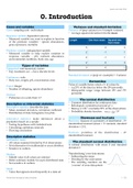
Cases and variables Variance and standard deviation
Cases: sampling unit - individuals Variance: σ2 (pop variance) or s2 (sample variance)
- Average squared deviation form the mean
Response variable: dependent outcome
- Measured variable you want to explain in function Length Dev from mean Squared dev
of the predictor variables - species abundances, from mean
gene expression, mortality
5 2 4
Predictor variable: independent variable
- Measured variable to help explain variation in 2 -1 1
response variable - pH, nutrient abundance, 2 -1 1
environmental conditions, body size, age
2 0 3
Types of variables
Categorical: non-numerical, factors 3 0 2
- Exp. treatment, sex → have discrete levels
Standard deviation: σ (pop) or s (sample) = √variance
Continuous: scale
- Body size, weight, pH, concentration, time
Percentiles
Value of variable below which x% of values lie
Count: integer - e.g 25% of the data lay below the 25th percentile
- Number of offspring, species abundance - Interquartile range: range between 25th and 75th
percentile
Ordinal:
- Preference on a scale from 1-7
The normal distribution
- Common distribution for continuous data
Descriptive vs inferential statistics - Bell-shaped, symmetrical around µ= x
Descriptive statistics: describe the data - Mean µ ± 1.96 * σ includes 95% of the observations
- Mean, standard deviation, correlation coefficient - Probability density function:
- Distribution of data, histograms, box plots
Inferential statistics: make inferences about a Skewness and kurtosis
population based on a sample Skewness: measure of asymmetry of distribution - 3rd
- Testing hypotheses with statistical tests standardized moment (mean = 1st moment, standard
- Calculating confidence intervals deviation = 2nd).
- Drawing conclusions
Kurtosis: pointless of the distribution - 4 th
standardized moment.
Descriptive statistics
(arithmetic) mean
- All values summed divided by # of observations The standard normal distribution
- Not informative for multimodal or asym distribut. A normal distribution with mean 0 and standard
- Sensitive to outliers deviation 1
Median ‘Standardizing’ your data means:
- Middle value if all values are ordered - Subtracting the mean
- Better summary statistic for asym distributed data - Dividing by the st.deviation
- Not sensitive to outliers - The resulting numbers are the
‘z-scores’ of your data points
Mode
- Value that appears most frequently in a data set
Advanced biological data analysis
, Laura van den End
Inferential statistics
We want to draw general conclusions about a
population based on sample
- Sample: part of pop that you studied
- Pop: all cases you could have studied
Standard error
When we calculate a statistic of a sample (e.g. the
mean), this is an estimate of that statistic for the
population. If we would sample again, we would get
a slightly different estimate every time. The standard
error is the standard deviation of that statistic across
our different samples
This is a measure of the precision that we have in
estimating the actual population statistic. We can
actually calculate this standard error based on just a
single sample: with n = Sample size.
Standard deviation vs standard error
The standard deviation is a measure of spread in our
sample ~ higher = more variability in the data.
The standard error is a measure of precision ~ higher
= the lower confidence in the accuracy of estimate.
- More data (the higher n) = lower the SE
- Confidence intervals are based on the SE
Using statistics to test hypotheses
H0: no effect, Q: can we reject H0 → when small
change to get our data, assuming H0 is true
Types of errors
Type I error (false positive) - we reject a true H0
- This is expected to happen in 5% of the cases!
- Multiple testing increases frequency
Type II error (false negative) - don’t reject false H0
- e.g. because sample size is too low (not enough
statistical power)
Note: we never accept or confirm H0 – we only do or
do not reject it
Advanced biological data analysis
, Laura van den End
1. Linear models
Continuous predictors Testing assumptions
STEP 1: visual inspection of raw data
> plot(body.length~heavy.metal.conc, data=caterpillars) Homogeneity of variances
STEP 2: regression line VISUALLY
- Draw the line → minimize the sum of squares of >spreadLevelPlot(fit3)
the difference between a datapoint and its - high absolute residuals = far away from reg. line
prediction - Low absolute residuals = close to regression line
- OLS - ordinaire least squares regression - We want equally distance. If the blue line is more
- Resulting line is given by 2 numbers: intercept and or less straight we have no problem.
slope:
TEST
>ncvTest(fit2)
STEP 3: fit a model → gives slope and intercept - If the p value is above 0.05 OK (no significant
> fit2 <- lm(body.length~heavy.metal.conc, data = data) deviation from homogeneous variances.
> summary(fit2)
NOT OK?
STEP 4: visualize results with effect plot - Transform data
>plot(allEffects(fit4), multiline = T, confint = list (style = - See if outliers
"auto")) - Use a model that allows for non-homogeneous
variances (gls)
STEP 5: hypothesis testing
- Take the summary table
- Take our confidence level given by SE Normality of residuals
- T value (estimate divided by SE) → more extreme
= less likely to get data if H0 is true VISUALLY
hist(rstudent(fit4), probability=T, ylim=c(0,0.5),
main="Distribution of Studentized Residuals",
Categorical predictors xlab="Studentized residuals”)
- Histogram of the studentized residuals of the
2 levels model
STEP 1 + 2 + 3 + 5: same
xfit=seq(-3,3, length=100)
STEP 4: same - Create a vector of X values for the normal
- R standard: ‘treatment coding’ = 1st alphabetical as distribution from -3 to 3
the reference level
- Sum coding → mean of all levels as reference level yfit=dnorm(xfit)
- Useful if collinearity in the data lines(xfit, yfit, col=“red”,lwd=2)
- Calculate and put values for a standard normal
More than 2 levels distribution of the range of x values given above
STEP 1 + 2 + 3 + 4: same
TEST
>shapiro.test(residuals(fit4))
STEP 5: check anova table for overall effect on the
- If W > 0.9 is OK
categorical predictor with more than 2 levels
> Anova(fit4, type=“III”)
Linearity
STEP 6: post-hoc comparisons >residualPlots(fit2)
- which levels of our predictor are different from - No strong relation is OK
each other?
> emmeans(fit4, ~samp.loc) Outliers and in uential observations
> contrast(emmeans(fit4, ~samp.loc), method='pairwise', > outlierTest(fit2) > cd <- cooks.distance(fit2)
adjust=‘Tukey’) > inflobs=which(cd>1);inflobs
Advanced biological data analysis
fl
The benefits of buying summaries with Stuvia:
Guaranteed quality through customer reviews
Stuvia customers have reviewed more than 700,000 summaries. This how you know that you are buying the best documents.
Quick and easy check-out
You can quickly pay through credit card or Stuvia-credit for the summaries. There is no membership needed.
Focus on what matters
Your fellow students write the study notes themselves, which is why the documents are always reliable and up-to-date. This ensures you quickly get to the core!
Frequently asked questions
What do I get when I buy this document?
You get a PDF, available immediately after your purchase. The purchased document is accessible anytime, anywhere and indefinitely through your profile.
Satisfaction guarantee: how does it work?
Our satisfaction guarantee ensures that you always find a study document that suits you well. You fill out a form, and our customer service team takes care of the rest.
Who am I buying these notes from?
Stuvia is a marketplace, so you are not buying this document from us, but from seller lauravandenend. Stuvia facilitates payment to the seller.
Will I be stuck with a subscription?
No, you only buy these notes for $6.95. You're not tied to anything after your purchase.