Module 3 : Frequency Control in a Power System
Lecture 12a : Solution of non-linear algebraic equations
Non-linear algebraic equations and their solution
In the next lecture, we will compute the steady state frequency of a power system, given the
load characteristics. We shall see that in general, this will require us to carry out a "loadflow".
A loadlfow involves the solution of a set of non-linear algebraic equations. Therefore, in this
lecture we revise the basic methods to solve non-linear algebraic equations.
We are aware that a transmission network in sinusoidal state state can be modelled by linear
algebraic equations in the node voltage phasors(V) and the nodal current phasor injections
(I):
where Ybus is the bus admittance matrix.
However, in power system studies, nodal injections are not specified as current phasors but as
real and reactive power injections (nonlinear functions of V and I) , and/or voltage
magnitudes of some nodes. We have also seen that real and reactive power can be a function
of frequency. In such a situation, obtaining the steady state solution (i.e. node voltage
phasors and frequency) will require us to solve a set of non-linear equations.
Therefore we take a silight diversion from the main theme and review why and how we use
numerical techniques for solving non-linear algebraic equations.
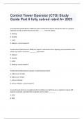
Let us consider the "why" question first. If we wish to solve an equation of the form:
Perhaps, "simplifying" it will help us solve it ?
Perhaps, if we take the natrual logarithm of both sides we may be able to do something ?
But soon enough you will realize that we seem to be getting nowhere !
It is clear that some other way (guess work ?) may be required to get the solution.
ixed Point Iteration Method
Since we have some idea of how the exponential function behaves we can try to guess the solution. We
know that:
, and
and
We can guess that the solution for should lie between 0.5 and 1.
However, this is a rough estimate. Surprisingly if we take an initial guess value :
and iterate as follows starting with k=0:
then x1=0.606, x2=0.545 , x3= 0.579, x4=0.5600, x5=0.571, x6=0.565, x7=0.568, x8=0.566, x9=0.567 ....
We seem to be "converging" to a solution which satisfies the equation !
Why does the Fixed Point Iterative Method Work ?
We can try to understand why we converge to the right solution by examining the behaviour of the iterative
method
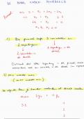
near the solution. Suppose the correct solution to the equation is x = xs , i.e.,
Suppose the value of x at the kth iteration is near the solution xs and differs from it by a small amount Dxk ,
i.e.,
then:
which yields :
therefore if at k=0, x = xinit then,
Since:
Lecture 12a : Solution of non-linear algebraic equations
Non-linear algebraic equations and their solution
In the next lecture, we will compute the steady state frequency of a power system, given the
load characteristics. We shall see that in general, this will require us to carry out a "loadflow".
A loadlfow involves the solution of a set of non-linear algebraic equations. Therefore, in this
lecture we revise the basic methods to solve non-linear algebraic equations.
We are aware that a transmission network in sinusoidal state state can be modelled by linear
algebraic equations in the node voltage phasors(V) and the nodal current phasor injections
(I):
where Ybus is the bus admittance matrix.
However, in power system studies, nodal injections are not specified as current phasors but as
real and reactive power injections (nonlinear functions of V and I) , and/or voltage
magnitudes of some nodes. We have also seen that real and reactive power can be a function
of frequency. In such a situation, obtaining the steady state solution (i.e. node voltage
phasors and frequency) will require us to solve a set of non-linear equations.
Therefore we take a silight diversion from the main theme and review why and how we use
numerical techniques for solving non-linear algebraic equations.
Let us consider the "why" question first. If we wish to solve an equation of the form:
Perhaps, "simplifying" it will help us solve it ?
Perhaps, if we take the natrual logarithm of both sides we may be able to do something ?
But soon enough you will realize that we seem to be getting nowhere !
It is clear that some other way (guess work ?) may be required to get the solution.
ixed Point Iteration Method
Since we have some idea of how the exponential function behaves we can try to guess the solution. We
know that:
, and
and
We can guess that the solution for should lie between 0.5 and 1.
However, this is a rough estimate. Surprisingly if we take an initial guess value :
and iterate as follows starting with k=0:
then x1=0.606, x2=0.545 , x3= 0.579, x4=0.5600, x5=0.571, x6=0.565, x7=0.568, x8=0.566, x9=0.567 ....
We seem to be "converging" to a solution which satisfies the equation !
Why does the Fixed Point Iterative Method Work ?
We can try to understand why we converge to the right solution by examining the behaviour of the iterative
method
near the solution. Suppose the correct solution to the equation is x = xs , i.e.,
Suppose the value of x at the kth iteration is near the solution xs and differs from it by a small amount Dxk ,
i.e.,
then:
which yields :
therefore if at k=0, x = xinit then,
Since: