Optimization I Notes Page 1
OPTIMIZATION I
Introduction – Lots of Geometry
Some definitions
o Definition (Convex set): The set Í n if convex if for any x1, x 2 Î and
l Î [0,1] , x(l) = lx1 + (1 - l)x 2 Î . Note that the intersection of a finite
number of convex sets is convex.
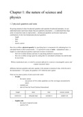
o Definition (Convex function): A function f (x ) defined on a convex set
Í n is convex if for any x1, x 2 Î , the linear interpolation between those two
points lies above the curve:
f (lx1 + (1 - l)x 2 ) £ l f (x1 ) + (1 - l)f (x 2 ) l Î [0,1]
x1 x2
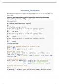
o Definition (Cone): A set Î n is a cone if for all x Î and any l ³ 0 ,
lx Î :
1
2
Daniel Guetta, 2010
,Optimization I Notes Page 2
{
The set x Î n : x = Aa, a ³ 0, A Î n´m , a Î m } is the cone generated by the
columns of A.
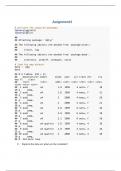
o Definition (extreme point): An extreme point of the convex set is a point
x Î that cannot be written as a convex combination of other points in .
Not an extreme point
Extreme point
Extreme point
o Definition (Convex Combination): A convex combination of points x1, , xk
is a point x = å i =1 li xi , such that l ³ 0 and å
k k
i =1
li = 1 . The set of convex
combinations of a set points is the smallest convex set containing all the points;
it is called the convex hull of these points.
o {
Definition (Hyperplane): The set = x Î n : a ⋅ x = b, a Î n , b Î } is
{
called a hyperplane with normal a. The set = x Î n : a ⋅ x £ b } is a closed
halfspace, and is its bounding hyperplane.
o Definition (Afine set): A set a Î n is an affine set if for all x1, x 2 Î a and
l Î (-¥, ¥) , x(l) = lx1 + (1 - l)x 2 Î a . A hyperplane is an example of an
affine set. Roughly speaking, an affine set is a subspace that need not contain the
original.
o Definition (Polyhedron): A polyhedron is a set which is the intersection of a
finite number of closed hyperplanes. It is necessarily convex. If the polyhedron is
non-empty and bounded (ie: there exists a large ball it lies inside of), it is called a
polytope.
o Definition (Dimension): The dimension of an affine set a is the maximum
number of linearly independent vectors in a .
o Definition (Supporting hyperplane): A supporting hyperplane of a closed,
convex set is a hyperplane such that Ç ¹ Æ and Í :
Daniel Guetta, 2010
,Optimization I Notes Page 3
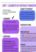
o Definition (Face): Let be a non-empty polyhedron and let be any
supporting hyperplane. The intersection Ç = is a face of . The whole
polyhedron could be a face, if the and are both two-dimensional! For
example, the thick line and the point in the example below are both faces of their
respective polyhedra:
2
1
We give special names to faces of particular dimensions:
Face Dimension
Vertex 0
Edge 1
Facet d–1
Another way of looking at the concept of a vertex is as a point x Î that is
such that there exists some c such that c ⋅ x < c ⋅ y for all y Î and y ¹ x . In
other words, we insist Ç =
= x . This simply means that our face is 0-
dimensional, and the definitions are therefore equivalent.
Daniel Guetta, 2010
, Optimization I Notes Page 4
Polyhedra in standard form
o The definition of a polyhedron above (in terms of the intersection of a number of
{
half-spaces) can be written as = Ax £ b : A Î n´m , x Î n , b Î m , where }
the rows of A contain the normals of the various hyperplanes defining the
polyhedron.
o It is often convenient, however, to write the polyhedron in an equivalent standard
{ ¢ ¢
}
form ¢ = A¢x = b : x ³ 0 , A Î n ´m , x Î n , b Î m , where the rows of A are
linearly independent. This involves a number of steps:
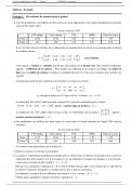
Re-write each inequality constraint Arow i ⋅ x £ bi as the equality
Arow i ⋅ x + si = bi , where si > 0. si becomes a new variable.
Eliminate any linearly independent rows in A (this does not alter the
problem – see page 57 of B&T for proof). Note that this implies that, in
standard form, m < n – in other words, the number of constraints is less
than or equal to the number of variables.)
Replace any unconstrained variables xi with two new variables x i+ and x i-
, both constrained to be positive, and add the constraint x i = x i+ - x i- .
[The validity of this step is not entirely obvious, but for the simplex
method, it works].
Algebraic Characterization of Vertices & Extreme Points
o In the previous section, we provided definitions of vertices and extreme points. It
would seem logical that the solution of a linear program should lie at one of these
points. In this section, we see that these concepts are equivalent, and we develop
an algebraic characterization of such points.
o We present two characterizations – the first is in terms of polyhedra in non-
standard form, which is more useful to gain an intuitive grasp of the concept, and
the second in terms of polyhedra in standard form, which we will use hereafter.
o Theorem: Let = {x : Ax ³ b, A¢x = b ¢} be a non-empty polyhedron, and let
x Î . The following three statements are equivalent:
1. x is a vertex
Daniel Guetta, 2010
OPTIMIZATION I
Introduction – Lots of Geometry
Some definitions
o Definition (Convex set): The set Í n if convex if for any x1, x 2 Î and
l Î [0,1] , x(l) = lx1 + (1 - l)x 2 Î . Note that the intersection of a finite
number of convex sets is convex.
o Definition (Convex function): A function f (x ) defined on a convex set
Í n is convex if for any x1, x 2 Î , the linear interpolation between those two
points lies above the curve:
f (lx1 + (1 - l)x 2 ) £ l f (x1 ) + (1 - l)f (x 2 ) l Î [0,1]
x1 x2
o Definition (Cone): A set Î n is a cone if for all x Î and any l ³ 0 ,
lx Î :
1
2
Daniel Guetta, 2010
,Optimization I Notes Page 2
{
The set x Î n : x = Aa, a ³ 0, A Î n´m , a Î m } is the cone generated by the
columns of A.
o Definition (extreme point): An extreme point of the convex set is a point
x Î that cannot be written as a convex combination of other points in .
Not an extreme point
Extreme point
Extreme point
o Definition (Convex Combination): A convex combination of points x1, , xk
is a point x = å i =1 li xi , such that l ³ 0 and å
k k
i =1
li = 1 . The set of convex
combinations of a set points is the smallest convex set containing all the points;
it is called the convex hull of these points.
o {
Definition (Hyperplane): The set = x Î n : a ⋅ x = b, a Î n , b Î } is
{
called a hyperplane with normal a. The set = x Î n : a ⋅ x £ b } is a closed
halfspace, and is its bounding hyperplane.
o Definition (Afine set): A set a Î n is an affine set if for all x1, x 2 Î a and
l Î (-¥, ¥) , x(l) = lx1 + (1 - l)x 2 Î a . A hyperplane is an example of an
affine set. Roughly speaking, an affine set is a subspace that need not contain the
original.
o Definition (Polyhedron): A polyhedron is a set which is the intersection of a
finite number of closed hyperplanes. It is necessarily convex. If the polyhedron is
non-empty and bounded (ie: there exists a large ball it lies inside of), it is called a
polytope.
o Definition (Dimension): The dimension of an affine set a is the maximum
number of linearly independent vectors in a .
o Definition (Supporting hyperplane): A supporting hyperplane of a closed,
convex set is a hyperplane such that Ç ¹ Æ and Í :
Daniel Guetta, 2010
,Optimization I Notes Page 3
o Definition (Face): Let be a non-empty polyhedron and let be any
supporting hyperplane. The intersection Ç = is a face of . The whole
polyhedron could be a face, if the and are both two-dimensional! For
example, the thick line and the point in the example below are both faces of their
respective polyhedra:
2
1
We give special names to faces of particular dimensions:
Face Dimension
Vertex 0
Edge 1
Facet d–1
Another way of looking at the concept of a vertex is as a point x Î that is
such that there exists some c such that c ⋅ x < c ⋅ y for all y Î and y ¹ x . In
other words, we insist Ç =
= x . This simply means that our face is 0-
dimensional, and the definitions are therefore equivalent.
Daniel Guetta, 2010
, Optimization I Notes Page 4
Polyhedra in standard form
o The definition of a polyhedron above (in terms of the intersection of a number of
{
half-spaces) can be written as = Ax £ b : A Î n´m , x Î n , b Î m , where }
the rows of A contain the normals of the various hyperplanes defining the
polyhedron.
o It is often convenient, however, to write the polyhedron in an equivalent standard
{ ¢ ¢
}
form ¢ = A¢x = b : x ³ 0 , A Î n ´m , x Î n , b Î m , where the rows of A are
linearly independent. This involves a number of steps:
Re-write each inequality constraint Arow i ⋅ x £ bi as the equality
Arow i ⋅ x + si = bi , where si > 0. si becomes a new variable.
Eliminate any linearly independent rows in A (this does not alter the
problem – see page 57 of B&T for proof). Note that this implies that, in
standard form, m < n – in other words, the number of constraints is less
than or equal to the number of variables.)
Replace any unconstrained variables xi with two new variables x i+ and x i-
, both constrained to be positive, and add the constraint x i = x i+ - x i- .
[The validity of this step is not entirely obvious, but for the simplex
method, it works].
Algebraic Characterization of Vertices & Extreme Points
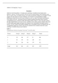
o In the previous section, we provided definitions of vertices and extreme points. It
would seem logical that the solution of a linear program should lie at one of these
points. In this section, we see that these concepts are equivalent, and we develop
an algebraic characterization of such points.
o We present two characterizations – the first is in terms of polyhedra in non-
standard form, which is more useful to gain an intuitive grasp of the concept, and
the second in terms of polyhedra in standard form, which we will use hereafter.
o Theorem: Let = {x : Ax ³ b, A¢x = b ¢} be a non-empty polyhedron, and let
x Î . The following three statements are equivalent:
1. x is a vertex
Daniel Guetta, 2010