Multivariate Statistics
Hyunmin Hong
October 18, 2023
1
,Contents
1 Lecture 1 4
1.1 Distance & Statistical Distance . . . . . . . . . . . . . . . . . . . . . . . . . . 4
1.2 Statistical Distance . . . . . . . . . . . . . . . . . . . . . . . . . . . . . . . . . 4
2 Lecture 2 6
2.1 Random Vectors & Random Matrices . . . . . . . . . . . . . . . . . . . . . . 6
2.2 Linear Combination of Random Vectors . . . . . . . . . . . . . . . . . . . . . 7
2.2.1 Univariate case . . . . . . . . . . . . . . . . . . . . . . . . . . . . . . . 7
2.2.2 Multivariate case . . . . . . . . . . . . . . . . . . . . . . . . . . . . . . 7
3 Lecture 3 8
3.1 Geometry of a Sample . . . . . . . . . . . . . . . . . . . . . . . . . . . . . . . 8
3.2 Geometric Interpretation of Average . . . . . . . . . . . . . . . . . . . . . . . 8
3.2.1 Deviation Vectors . . . . . . . . . . . . . . . . . . . . . . . . . . . . . 9
3.3 Estimation of µ & Σ . . . . . . . . . . . . . . . . . . . . . . . . . . . . . . . . 10
4 Lecture 4 12
4.1 Generalized Variance . . . . . . . . . . . . . . . . . . . . . . . . . . . . . . . . 12
4.1.1 Generalized Variance in p dimensions . . . . . . . . . . . . . . . . . . 13
4.2 Geometric Interpretation of Statistical Distance . . . . . . . . . . . . . . . . . 14
4.3 Geometric Intuition of Covariance Matrix . . . . . . . . . . . . . . . . . . . . 15
5 Lecture 5 16
5.1 Multivariate Normal Distribution . . . . . . . . . . . . . . . . . . . . . . . . . 16
5.1.1 Properties of Multivariate Normal Distribution . . . . . . . . . . . . . 17
6 Lecture 6 22
6.1 Estimation (by Maximum Likelihood) . . . . . . . . . . . . . . . . . . . . . . 22
6.1.1 Maximum Likelihood Estimates . . . . . . . . . . . . . . . . . . . . . . 22
7 Lecture 7 23
7.1 MLE of Multivariate Normal Distribution . . . . . . . . . . . . . . . . . . . . 23
7.1.1 Remarks about MLE . . . . . . . . . . . . . . . . . . . . . . . . . . . . 26
7.1.2 What is the distribution of µ̂M LE & Σ̂M LE ? . . . . . . . . . . . . . . 26
8 Lecture 8 27
8.1 Asymptotic Behavior of µ̂M LE & Σ̂M LE . . . . . . . . . . . . . . . . . . . . . 27
8.2 Data Inspection and Distributional Assumptions Check . . . . . . . . . . . . 27
8.2.1 Transformations . . . . . . . . . . . . . . . . . . . . . . . . . . . . . . 28
8.3 Multivariate Tests . . . . . . . . . . . . . . . . . . . . . . . . . . . . . . . . . 29
8.3.1 Univariate Tests . . . . . . . . . . . . . . . . . . . . . . . . . . . . . . 29
8.3.2 Multivariate Tests (of location, µ) . . . . . . . . . . . . . . . . . . . . 29
9 Lecture 9 30
9.1 Invariance Property of Hotelling’s T 2 . . . . . . . . . . . . . . . . . . . . . . . 30
9.2 Likelihood Ratio Tests (LRT) . . . . . . . . . . . . . . . . . . . . . . . . . . . 31
9.3 Equivalence of Hotelling’s T 2 & Wilks’ Lambda . . . . . . . . . . . . . . . . . 32
10 Lecture 10 33
10.1 Confidence Regions . . . . . . . . . . . . . . . . . . . . . . . . . . . . . . . . . 33
2
, 10.2 Simultaneously Valid Confidence Intervals . . . . . . . . . . . . . . . . . . . . 33
10.2.1 Correction for Simultaneous Validity . . . . . . . . . . . . . . . . . . . 34
10.2.2 Simultaneously Valid Individual Confidence Intervals . . . . . . . . . . 34
10.3 Bonferroni Correction . . . . . . . . . . . . . . . . . . . . . . . . . . . . . . . 35
10.4 Asymptotic Approximation . . . . . . . . . . . . . . . . . . . . . . . . . . . . 35
11 Lecture 11 37
11.1 Principal Component Analysis . . . . . . . . . . . . . . . . . . . . . . . . . . 37
11.1.1 Properties & Interpretation of principal components . . . . . . . . . . 38
12 Lecture 12 40
12.1 Principal Component Analysis (continued) . . . . . . . . . . . . . . . . . . . . 40
12.1.1 Principal components are not scale invariant . . . . . . . . . . . . . . 40
12.1.2 Special Cases . . . . . . . . . . . . . . . . . . . . . . . . . . . . . . . . 41
12.1.3 How many principal components to retain? . . . . . . . . . . . . . . . 42
12.2 Factor Analysis . . . . . . . . . . . . . . . . . . . . . . . . . . . . . . . . . . . 42
13 Lecture 13 44
13.1 Factor Analysis (continued) . . . . . . . . . . . . . . . . . . . . . . . . . . . . 44
13.1.1 Estimation of L & Ψ . . . . . . . . . . . . . . . . . . . . . . . . . . . . 45
13.1.2 Estimation of Factor Scores . . . . . . . . . . . . . . . . . . . . . . . . 46
13.1.3 How to choose # of factors? . . . . . . . . . . . . . . . . . . . . . . . . 47
3
, 1 Lecture 1
1.1 Distance & Statistical Distance
Definition 1.1. Distance is a function defined on M .
d(x, y) : M × M → R
such that
a) d(x, y) ≥ 0, d(x, y) = 0 if x = y.
b) d(x, y) = d(y, x) (symmetry)
c) d(x, z) ≤ d(x, y) + d(y, z) (triangle inequality)
Example 1.1 (Euclidean distance).
p
d(x, y) = (x1 − y1 )2 + (x2 − y2 )2
△
Example 1.2 (Manhattan distance).
d(x, y) = |x1 − y1 | + |x2 − y2 |
△
1.2 Statistical Distance
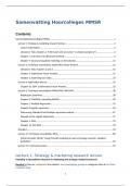
Intuition. You might think that the red square is more extreme from the mean value
than blue square since it does not fall within the cloud of points. However, their Euclidean
distances are equal. Hence, we must take the variance into account when the cloud of
points is distributed in ellipse shape.
4
Hyunmin Hong
October 18, 2023
1
,Contents
1 Lecture 1 4
1.1 Distance & Statistical Distance . . . . . . . . . . . . . . . . . . . . . . . . . . 4
1.2 Statistical Distance . . . . . . . . . . . . . . . . . . . . . . . . . . . . . . . . . 4
2 Lecture 2 6
2.1 Random Vectors & Random Matrices . . . . . . . . . . . . . . . . . . . . . . 6
2.2 Linear Combination of Random Vectors . . . . . . . . . . . . . . . . . . . . . 7
2.2.1 Univariate case . . . . . . . . . . . . . . . . . . . . . . . . . . . . . . . 7
2.2.2 Multivariate case . . . . . . . . . . . . . . . . . . . . . . . . . . . . . . 7
3 Lecture 3 8
3.1 Geometry of a Sample . . . . . . . . . . . . . . . . . . . . . . . . . . . . . . . 8
3.2 Geometric Interpretation of Average . . . . . . . . . . . . . . . . . . . . . . . 8
3.2.1 Deviation Vectors . . . . . . . . . . . . . . . . . . . . . . . . . . . . . 9
3.3 Estimation of µ & Σ . . . . . . . . . . . . . . . . . . . . . . . . . . . . . . . . 10
4 Lecture 4 12
4.1 Generalized Variance . . . . . . . . . . . . . . . . . . . . . . . . . . . . . . . . 12
4.1.1 Generalized Variance in p dimensions . . . . . . . . . . . . . . . . . . 13
4.2 Geometric Interpretation of Statistical Distance . . . . . . . . . . . . . . . . . 14
4.3 Geometric Intuition of Covariance Matrix . . . . . . . . . . . . . . . . . . . . 15
5 Lecture 5 16
5.1 Multivariate Normal Distribution . . . . . . . . . . . . . . . . . . . . . . . . . 16
5.1.1 Properties of Multivariate Normal Distribution . . . . . . . . . . . . . 17
6 Lecture 6 22
6.1 Estimation (by Maximum Likelihood) . . . . . . . . . . . . . . . . . . . . . . 22
6.1.1 Maximum Likelihood Estimates . . . . . . . . . . . . . . . . . . . . . . 22
7 Lecture 7 23
7.1 MLE of Multivariate Normal Distribution . . . . . . . . . . . . . . . . . . . . 23
7.1.1 Remarks about MLE . . . . . . . . . . . . . . . . . . . . . . . . . . . . 26
7.1.2 What is the distribution of µ̂M LE & Σ̂M LE ? . . . . . . . . . . . . . . 26
8 Lecture 8 27
8.1 Asymptotic Behavior of µ̂M LE & Σ̂M LE . . . . . . . . . . . . . . . . . . . . . 27
8.2 Data Inspection and Distributional Assumptions Check . . . . . . . . . . . . 27
8.2.1 Transformations . . . . . . . . . . . . . . . . . . . . . . . . . . . . . . 28
8.3 Multivariate Tests . . . . . . . . . . . . . . . . . . . . . . . . . . . . . . . . . 29
8.3.1 Univariate Tests . . . . . . . . . . . . . . . . . . . . . . . . . . . . . . 29
8.3.2 Multivariate Tests (of location, µ) . . . . . . . . . . . . . . . . . . . . 29
9 Lecture 9 30
9.1 Invariance Property of Hotelling’s T 2 . . . . . . . . . . . . . . . . . . . . . . . 30
9.2 Likelihood Ratio Tests (LRT) . . . . . . . . . . . . . . . . . . . . . . . . . . . 31
9.3 Equivalence of Hotelling’s T 2 & Wilks’ Lambda . . . . . . . . . . . . . . . . . 32
10 Lecture 10 33
10.1 Confidence Regions . . . . . . . . . . . . . . . . . . . . . . . . . . . . . . . . . 33
2
, 10.2 Simultaneously Valid Confidence Intervals . . . . . . . . . . . . . . . . . . . . 33
10.2.1 Correction for Simultaneous Validity . . . . . . . . . . . . . . . . . . . 34
10.2.2 Simultaneously Valid Individual Confidence Intervals . . . . . . . . . . 34
10.3 Bonferroni Correction . . . . . . . . . . . . . . . . . . . . . . . . . . . . . . . 35
10.4 Asymptotic Approximation . . . . . . . . . . . . . . . . . . . . . . . . . . . . 35
11 Lecture 11 37
11.1 Principal Component Analysis . . . . . . . . . . . . . . . . . . . . . . . . . . 37
11.1.1 Properties & Interpretation of principal components . . . . . . . . . . 38
12 Lecture 12 40
12.1 Principal Component Analysis (continued) . . . . . . . . . . . . . . . . . . . . 40
12.1.1 Principal components are not scale invariant . . . . . . . . . . . . . . 40
12.1.2 Special Cases . . . . . . . . . . . . . . . . . . . . . . . . . . . . . . . . 41
12.1.3 How many principal components to retain? . . . . . . . . . . . . . . . 42
12.2 Factor Analysis . . . . . . . . . . . . . . . . . . . . . . . . . . . . . . . . . . . 42
13 Lecture 13 44
13.1 Factor Analysis (continued) . . . . . . . . . . . . . . . . . . . . . . . . . . . . 44
13.1.1 Estimation of L & Ψ . . . . . . . . . . . . . . . . . . . . . . . . . . . . 45
13.1.2 Estimation of Factor Scores . . . . . . . . . . . . . . . . . . . . . . . . 46
13.1.3 How to choose # of factors? . . . . . . . . . . . . . . . . . . . . . . . . 47
3
, 1 Lecture 1
1.1 Distance & Statistical Distance
Definition 1.1. Distance is a function defined on M .
d(x, y) : M × M → R
such that
a) d(x, y) ≥ 0, d(x, y) = 0 if x = y.
b) d(x, y) = d(y, x) (symmetry)
c) d(x, z) ≤ d(x, y) + d(y, z) (triangle inequality)
Example 1.1 (Euclidean distance).
p
d(x, y) = (x1 − y1 )2 + (x2 − y2 )2
△
Example 1.2 (Manhattan distance).
d(x, y) = |x1 − y1 | + |x2 − y2 |
△
1.2 Statistical Distance
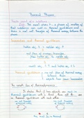
Intuition. You might think that the red square is more extreme from the mean value
than blue square since it does not fall within the cloud of points. However, their Euclidean
distances are equal. Hence, we must take the variance into account when the cloud of
points is distributed in ellipse shape.
4