Complete summary of all content of the Statistical Modelling in Medical Research course (BMs61). This includes a clear description of linear regression and logistic regression, as well as two types of variable selection; backwards elimination and forward selection. The summary provides a descriptio...
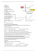
Y = dependent variable
B0 = intercept (or starting value)
B1 = Slope
X = independent variable (or amount)
E = random error
Least squared method
To know the best fitted line (smallest SSE)
R^2 : Explains proportion of
variance in de dependent variable
that can be explained by the
independent variable.
R^2 = (SSY – SSE) / SSY
Close to 1 is perfect (meaning low
SSE).
R^2 = (correlation coefficient)^2
Dummy variable and comparing regression lines
Use dummy variables to study whether the relationship between two variables is different across
subgroups of a population.
If there are k categories, there are k-1 dummy variables
Time = B0 + B1*Z + B2*age + B3*Z*age + E (met Z = 0 male and Z = 1 female)
Males TIME = B0 + B1*0 + B2*age + B3*0*age + E = B0 + B1*age + E
Females TIME = B0 + B1*1 + B2*age + B3*1*age + E = B0 + B1 + B2*age + B3*age
So for males the intercept is B0 and the slope is B1*age, while for females the intercept is B0+B1 and
the slope is B2*age + B3*age. This results in different intercept and slope for males/females.
Testing hypothesis using Time = B0 + B1*Z + B2*age + B3*Z*age + E (met Z = 0 m and Z = 1 f)
How do you test if there is different association between men and female?
H0 = there is no difference or B3 = 0 (meaning interaction term/effect modification isn’t there)
How do you test if the model explains the data better than the empty model?
H0 = there is no difference or B1 = B2 = B3 = 0
Overall F-test
Compare model with no predictor to model with predictors
Y = B0 + E
Y = B0 + B1*X + B2*W + B3*Z + E H0: B1 = B2 = B3 = 0
F = ((SSY-SSE)/k) / (SSE/(n-k-1)) n = n of observations k = n of predictors
Results in F-test with p-value. If p-value < significance new model fits data better.
, Partial F-test
Compares model with k predictors (reduced) to a model with k+m predictors (full)
Y = B0 + B1*X + B2*W + E
Y = B0 + B1*X + B2*W + B3*Z + E H0: B3 = 0
F = ((SSEredu-SSEfull)/m) / (SSEfull/(n-(k+m)-1))
k = n of predictors in reduced model
k+m = n of predictors in the full model
n = n of observations
Results in F-test with p-value. If p-value < significance new model fits data better.
T-test
Compares model with k predictors (reduced) to a model with k+1 predictors (full)
So t-test can be used when the difference in predictors between the two models is 1. T-test evaluates
B estimates, while F-test evaluates the residuals (using SSE).
Homoscedasticity: Assumption that equal or similar variances are present in the different groups
being compared. This and linearity are both assumptions of linear regression. So often data is ln
transformed to make it normal and thus be able to assume homoscedasticity.
WEEK 2
How do you deal with Confounding?
I. Stratification
Divide date into groups
BP = B0 + B1*bmi + E (unadj.)
BP = B<30 + B<30*bmi + E (adj. for
BP = B>30 + B>30*bmi + E subgroups)
Problem with this: Reduction in sample sizes and usually not possible for several confounders at the
same time.
II. Include confounder in model
Add it into the model as addition to the predictor variables of interest. Then the effect of variables of
interest is adjusted/controlled for the effect of the confounder.
BP = B0 + B1*bmi + E (unadj.)
BP = B0 + B1*bmi + B2*Z + E (adj.)
You use dummy variable (Z) to adjust.
Or add confounder as continuous variable (age).
BP = B0 + B1*bmi + E (unadj.)
BP = B0 + B1*bmi + B2*age + E (adj.)
If the change from B1 to B1 is >10%, this change is meaningful, meaning there may be confounding.
The benefits of buying summaries with Stuvia:
Guaranteed quality through customer reviews
Stuvia customers have reviewed more than 700,000 summaries. This how you know that you are buying the best documents.
Quick and easy check-out
You can quickly pay through credit card or Stuvia-credit for the summaries. There is no membership needed.
Focus on what matters
Your fellow students write the study notes themselves, which is why the documents are always reliable and up-to-date. This ensures you quickly get to the core!
Frequently asked questions
What do I get when I buy this document?
You get a PDF, available immediately after your purchase. The purchased document is accessible anytime, anywhere and indefinitely through your profile.
Satisfaction guarantee: how does it work?
Our satisfaction guarantee ensures that you always find a study document that suits you well. You fill out a form, and our customer service team takes care of the rest.
Who am I buying these notes from?
Stuvia is a marketplace, so you are not buying this document from us, but from seller rdkmn. Stuvia facilitates payment to the seller.
Will I be stuck with a subscription?
No, you only buy these notes for $12.31. You're not tied to anything after your purchase.