100% satisfaction guarantee Immediately available after payment Both online and in PDF No strings attached
logo-home
ARMA Model - Stata Lab Session Notes $5.96   Add to cart

Class notes

ARMA Model - Stata Lab Session Notes

 271 views  0 purchase
  • Course
  • Institution

Here are the notes from the ARMA Model Lab session. The document includes all the steps with the explanation attached. There are 8 steps. 1 - Looking to the data, 2 - Looking at the autocorrelation plot, 3 - Estimate ARMA models, 4 - Construct residuals and check if there is autocorrelation, 5 - C...

[Show more]
Preview 10 out of 20  pages

  • November 28, 2017
  • 20
  • 2017/2018
  • Class notes
  • Unknown
  • All classes
avatar-seller
ARMA Model – Stata Lab Session Notes


1st Step – Looking to the data
.1
.08
.06
Density


.04
.02
0


0 20 40 60 80
VIX


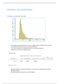
- The histogram is important because if we use an ARMA model for modeling VIX you assume
a normal distribution because you use maximum likelihood.
- In our case is important to note that the series is not normally distributed.
- Formally we can test this by typing sktest VIX


- Skewness should be 0 and kurtosis should be 3  in our case we reject the H0 of normally
distributed variable.
- We already expect this because we saw the histogram.

, 2nd Step – Looking at the autocorrelation plot


Autocorrelation Partial Autocorrelation


1.00
1.00


0.80
Partial autocorrelations of VIX
0.50


0.60
0.40
0.00


0.20
0.00
-0.50


0 10 20 30 40 0 10 20 30 40
Lag Lag
Bartlett's formula for MA(q) 95% confidence bands 95% Confidence bands [se = 1/sqrt(n)]


// make a plot of the (partial) autocorrelations

ac VIX in 1/1511, name(ACplot)

pac VIX in 1/1511, name(PACplot)

- We now look at an in-sample period  (1511 days)
o You can take also half of the data and test the model on the other half.

What do we see?

- Autocorrelation declines very slowly.
- Partial autocorrelation is almost zero after lag 1 or 2 or 3 .
- This is more AR type of model than MA.
o The reason is because MA says that the autocorrelation will drop immediate to zero
after certain lag. Here it is not the case.
o AR, on the other hand, says that the partial autocorrelation drops to zero and you
can see it in the graph. However, the autocorrelation alone does not decline
exponentially to zero.
- If you see this two plots, you should think that this is more a type of AR MA model but it is
not completely AR  therefore we should go for an ARMA model.

, 3rd Step – Estimate ARMA models

//estimate various ARMA models

arima VIX in 1/1511, ar(1/1) ma(1/1)

estat acplot, name(theoACarma11)

arima VIX in 1/1511, ar(1/2) ma(1/1)

estat acplot, name(theoACarma21)


AR(2,1)
ARIMA regression

Sample: 1 - 1511 Number of obs = 1511
Wald chi2(3) = 1.27e+06
Log likelihood = -3068.989 Prob > chi2 = 0.0000


OPG
VIX Coef. Std. Err. z P>|z| [95% Conf. Interval]

VIX
_cons 20.27916 8.485587 2.39 0.017 3.647713 36.9106

ARMA
ar
L1. 1.442787 .0397349 36.31 0.000 1.364908 1.520666
L2. -.4459915 .0392521 -11.36 0.000 -.5229243 -.3690588

ma
L1. -.6463761 .03225 -20.04 0.000 -.709585 -.5831672

/sigma 1.842184 .0119603 154.03 0.000 1.818743 1.865626

Note: The test of the variance against zero is one sided, and the two-sided
confidence interval is truncated at zero.


- Coefficients = 1.44 and -0.44.
- Remember that Ф1 + Ф2 should not exceed 1  here is 0.9967955

 Immediately after you estimate the model compute estat ic, n(1511) to look at the AIC and BIC

, - You can’t do anything with the values at the moment because you must compare it with
various models.


AR(1)


- Coefficients = 0.9913489 and -0.2075646.
- Remember that Ф1 + Ф2 should not exceed 1  here is 0.7837843
o This is exactly what we previous thought because the autocorrelations looks almost
like a random walk  like an AR1 with the values of 1.


 Immediately after you estimate the model compute estat ic, n(1511) to look at the AIC and BIC

, . estat ic, n(1511)

Akaike's information criterion and Bayesian information criterion


Model Obs ll(null) ll(model) df AIC BIC

. 1,511 . -3068.989 5 6147.978 6174.58

Note: N=1511 used in calculating BIC.


- After comparing the AIC and BIC we can conclude that AR (2,1) model has lower values than
AR(1). So, AR(2,1) is better.
- The differences are not that big.
- AR(1) has higher AIC and BIC than AR(2)
o This is because the model look almost like a random walk.
o An AR(1) model with Ф = 0.99 is almost a random walk.
- What you learn from this is that if you see an AC or PAC and you see that is quite close to a
certain model then you already know that if you use other models for forecasting.

4th Step – Construct residuals and check if there is autocorrelation

predict resARMA11 in 1/1511, residuals // make residuals

ac resARMA11 in 1/1511, name(ACresARMA11) //plot autocorrelations of the residuals

wntestq resARMA11 in 1/1511, lags(5)

- Until now we estimated the model.
- However, after you do this, you want to check if the model is ok so you check its residuals.
- You create a new variable with the code above.
0.10
0.05
Autocorrelations of AR1


0.00
-0.05
-0.10


0 10 20 30 40
Lag
Bartlett's formula for MA(q) 95% confidence bands

, - You can see that there are 1,970 missing values generated.
- Be careful always to specify you sample in the code.
- This graph does not look good because we see significantly autocorrelation in lag 1, lag 3,
and lag 5.
- Next, we run a test to confirm our outcome


- The F test is very high 41.36, and the p-value is zero.
- We can reject the H0 hypothesis that there is no autocorrelation.
o The test tells us that there is indeed autocorrelation in the residuals.

Conclusion: ARMA (1) has autocorrelation if the residuals. Therefore, let’s look at ARMA (2,1)

AR(2,1)
0.10
Autocorrelations of resARMA12


0.05
0.00
-0.05
-0.10


0 10 20 30 40
Lag
Bartlett's formula for MA(q) 95% confidence bands


- Be careful because you must estimate the model again and change the cod accordingly to fit
with ARMA (2,1)
- The graph looks slightly better than the previous one because I do not see the negative
significant autocorrelation in lag1 anymore.
- We can see something at lag3 and lag 5.
- We run the test again.

, - The F test is also high 27.83, and the p-value is zero but slightly lower than the previous one.
- Also here, we can reject the H0 hypothesis that there is no autocorrelation.
o The test tells us that there is indeed autocorrelation in the residuals.

Conclusion: ARMA (2,1) has autocorrelation if the residuals.


5th Step – Construct the fit of the model

arima VIX in 1/1511, ar(1/1) ma(1/1)

predict fitARMA11 in 1/1511, xb

twoway (line VIX time in 1/1511) (line fitARMA11 time in 1/1511)

AR(1)
80
60
40
20
0


0 500 1000 1500
time

VIX xb prediction, one-step


- The fit of the model looks amazing.
- We see the red line, but we don’t see the blue line anymore.
- The blue line is the original series and the red line is the fit of the 1150 observations.

,AR(2,1)
80
60
40
20
0


0 500 1000 1500
time

VIX xb prediction, one-step


- In terms of fit, we did an extremely good job.

Why does the fit looks so good?

- It is because these time series are full of autocorrelation.


Additional Steps – Test for homoscedasticity

gen res2ARMA11 = resARMA11^2

ac res2ARMA11 in 1/1511, name(ACres2ARMA11)

- We assume from all the ARMA models that the variance of the error terms had a mean of
zero and a variance of σ2 so it is constant.
- You can check whether is true for the VIX while computing the squared residuals (check the
code).

, 0.60
0.40
0.20
0.00
-0.20


0 10 20 30 40
Lag
Bartlett's formula for MA(q) 95% confidence bands


- Huge autocorrelation in squared residuals.
- The squared residuals of today have a lot to do with the squared residuals of yesterday.
- The graph shows that there is heteroscedasticity. The implication of heteroscedasticity is
that is harming the standard error of the coefficients. So, this is bad for the model.


Additional Steps – Log of VIX

- We saw previously that the series was not normally distributed.
- In this case we can compute the log of the VIX

gen lnVIX = ln(VIX)

arima lnVIX in 1/1511, ar(1/1) ma(1/1)

predict ehat_LN_arma11, residuals

gen ehat2_LN_arma11 = ehat_LN_arma11^2

ac ehat2_LN_arma11, name(ACres2ARMA_LOG)

graph combine ACres2ARMA11 ACres2ARMA_LOG

, Autocorrelation Partial Autocorrelation


1.00
1.00


0.80
Partial autocorrelations of VIX
0.50


0.60
0.40
0.00


0.20
0.00
-0.50


0 10 20 30 40 0 10 20 30 40
Lag Lag
Bartlett's formula for MA(q) 95% confidence bands 95% Confidence bands [se = 1/sqrt(n)]


- It looks almost the same at the first ones.


 Estimate the model but for the log of the VIX

AR(2,1)


- Coefficients = 1.509166 and -0.5116233

The benefits of buying summaries with Stuvia:

Guaranteed quality through customer reviews

Guaranteed quality through customer reviews

Stuvia customers have reviewed more than 700,000 summaries. This how you know that you are buying the best documents.

Quick and easy check-out

Quick and easy check-out

You can quickly pay through credit card or Stuvia-credit for the summaries. There is no membership needed.

Focus on what matters

Focus on what matters

Your fellow students write the study notes themselves, which is why the documents are always reliable and up-to-date. This ensures you quickly get to the core!

Frequently asked questions

What do I get when I buy this document?

You get a PDF, available immediately after your purchase. The purchased document is accessible anytime, anywhere and indefinitely through your profile.

Satisfaction guarantee: how does it work?

Our satisfaction guarantee ensures that you always find a study document that suits you well. You fill out a form, and our customer service team takes care of the rest.

Who am I buying these notes from?

Stuvia is a marketplace, so you are not buying this document from us, but from seller claudiughiuzan. Stuvia facilitates payment to the seller.

Will I be stuck with a subscription?

No, you only buy these notes for $5.96. You're not tied to anything after your purchase.

Can Stuvia be trusted?

4.6 stars on Google & Trustpilot (+1000 reviews)

77254 documents were sold in the last 30 days

Founded in 2010, the go-to place to buy study notes for 14 years now

Start selling
$5.96
  • (0)
  Add to cart