Lecture 1
05-02-2019
Chapter 5: Introduction to Risk, Return and the Historical Record
Return
𝐷𝑖𝑡 + 𝑃𝑖𝑡 − 𝑃𝑖𝑡−1
Return = = 𝑅𝑖𝑡 = 𝐻𝑃𝑅
𝑃𝑖𝑡−1
→ How much is the price changing with respect to an earlier price?
Expected Return
𝐸[𝑅𝑖𝑡 ] = Expected HPR
→ The return you expect the index to have. You can use historical data to tell something about the
expected return.
P0 = 100
120 probability = ½
P1
90 probability = ½
E[R] = ½ x 120 + ½ x 90 = 60 + 45 = 105
Example:
Probability Value
0,1 2
0,2 3 Expected value = 0.1 x 2 + 0.2 x 3 + 0.2 x 9 + 0.5 x 8 = 6.6
0,2 9 → Use SOMPRODUCT/SUMPRODUCT in excel
0,5 8
Excess Return
Excess Return = 𝑅𝑖𝑡 − 𝑟𝑓
→ The difference between putting money in a risk-free asset or putting it in an asset with risk.
If the calculation is equal to 0, you invest in the risk-free asset.
Risk Premium
Risk Premium = E[𝑅𝑖𝑡 ] − 𝑟𝑓
→ Basically the money that you want to be compensated for taking risk.
Some statistics
• Mean: 𝜇𝑖 = 𝐸[𝑅𝑖𝑡 ]
• Variance: 𝜎𝑖2 = 𝐸[(𝑅𝑖𝑡 − 𝜇𝑖 )2 ]
• Standard deviation: 𝜎𝑖 = √𝜎𝑖2
Other (relevant) statistics
• Covariance: 𝐸[𝑅𝑖𝑡 − 𝜇𝑖 ) − (𝑟𝑗𝑡 − 𝜇𝑗 )]
𝐸[𝑅𝑖𝑡 −𝜇𝑖 )−(𝑟𝑗𝑡 −𝜇𝑗 )]
• Correlation:
𝜎𝑖 𝜎𝑗
Both capture how variables move together
1
, (a) Skewness characterizes the degree of asymmetry of a distribution around its mean. It is a pure number
that characterizes only the shape of the distribution
1 𝑋𝑠 −𝑋̅ 3
a. Skewnness = ∑𝑛𝑠=1 [ ]
n 𝜎
(b) Kurtosis measures the size of a distribution’s tails. For a heavy-tailed distribution, probability mass
shifts from the intermediate parts of the distribution to both the tails and the middle.
1 𝑋𝑠 −𝑋̅ 4
a. Kurtosis = { ∑𝑛𝑠=1 [ ] }−3
n 𝜎
Note: Kurtosis is a non-dimensional measure
Can you think of any implications from an investor’s point of view?
→ You are not able to tell what happens in extreme cases
Why Normal Distribution?
• Well-behaving distribution
• Stability
• Additivity
Is “It” Worth It?
Risk Premium
Sharpe Ratio =
𝜎(Excess Return)
→ Looks at the tradeoff between risk and return. This is what an investor is interested in. How attractive
is a portfolio or a certain index?
Note: The annualized Sharpe Ratio is obtained when multiplying the Sharpe Ratio times √12
Other risk measures … Value-At-Risk/VaR
• Quantifies the total risk of an investment portfolio
• Pioneered by JPMorgan
• We are X% certain that we will not lose more than $V in time T
• Use the probability distribution of gains (losses) during time T
2
, Example: Value-At-Risk/VaR
Suppose the change in the value of an MNC’s portfolio over a 10-day time horizon is normally distributed with
a mean of zero and a standard deviation of $20 MM. What is the 10-day 99% VaR?
VaR = σN −1 (𝑋)
Note: This VaR measure is expressed in USD
Excel: NORM.INV
Answer: VaR = $20MM N-1(0.99) = 20MM x (2.326) = $46.53MM
Chapters 6 + 7: Capital Allocation to Risky Assets & Optimal Risky Portfolios
Mean Variance Analysis
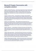
• Various point showing different E[rp] and p combinations providing equal utility to the investor
• How does the indifference curve of a less/more risk-averse investor compare to this indifference
curve?
Mean Variance Analysis
Which investor has a risk aversion coefficient equal to 4?
The higher level of U, the more risk averse someone is. Higher risk aversion index, higher the coefficient. 4 =
steeper line. X is risk y is return.
Basic Properties of Mean and Variance for Portfolio Returns
𝑅𝑃 = 𝑤1 𝑅1 + 𝑤2 𝑅2 + ⋯ + 𝑤1−𝑛 𝑅1−𝑛 + 𝑤𝑛 𝑅𝑛
𝐸[𝑅𝑃 ] = 𝑤1 𝜇1 + 𝑤2 𝜇2 + ⋯ + 𝑤1−𝑛 𝜇1−𝑛 + 𝑤𝑛 𝜇𝑛
3
05-02-2019
Chapter 5: Introduction to Risk, Return and the Historical Record
Return
𝐷𝑖𝑡 + 𝑃𝑖𝑡 − 𝑃𝑖𝑡−1
Return = = 𝑅𝑖𝑡 = 𝐻𝑃𝑅
𝑃𝑖𝑡−1
→ How much is the price changing with respect to an earlier price?
Expected Return
𝐸[𝑅𝑖𝑡 ] = Expected HPR
→ The return you expect the index to have. You can use historical data to tell something about the
expected return.
P0 = 100
120 probability = ½
P1
90 probability = ½
E[R] = ½ x 120 + ½ x 90 = 60 + 45 = 105
Example:
Probability Value
0,1 2
0,2 3 Expected value = 0.1 x 2 + 0.2 x 3 + 0.2 x 9 + 0.5 x 8 = 6.6
0,2 9 → Use SOMPRODUCT/SUMPRODUCT in excel
0,5 8
Excess Return
Excess Return = 𝑅𝑖𝑡 − 𝑟𝑓
→ The difference between putting money in a risk-free asset or putting it in an asset with risk.
If the calculation is equal to 0, you invest in the risk-free asset.
Risk Premium
Risk Premium = E[𝑅𝑖𝑡 ] − 𝑟𝑓
→ Basically the money that you want to be compensated for taking risk.
Some statistics
• Mean: 𝜇𝑖 = 𝐸[𝑅𝑖𝑡 ]
• Variance: 𝜎𝑖2 = 𝐸[(𝑅𝑖𝑡 − 𝜇𝑖 )2 ]
• Standard deviation: 𝜎𝑖 = √𝜎𝑖2
Other (relevant) statistics
• Covariance: 𝐸[𝑅𝑖𝑡 − 𝜇𝑖 ) − (𝑟𝑗𝑡 − 𝜇𝑗 )]
𝐸[𝑅𝑖𝑡 −𝜇𝑖 )−(𝑟𝑗𝑡 −𝜇𝑗 )]
• Correlation:
𝜎𝑖 𝜎𝑗
Both capture how variables move together
1
, (a) Skewness characterizes the degree of asymmetry of a distribution around its mean. It is a pure number
that characterizes only the shape of the distribution
1 𝑋𝑠 −𝑋̅ 3
a. Skewnness = ∑𝑛𝑠=1 [ ]
n 𝜎
(b) Kurtosis measures the size of a distribution’s tails. For a heavy-tailed distribution, probability mass
shifts from the intermediate parts of the distribution to both the tails and the middle.
1 𝑋𝑠 −𝑋̅ 4
a. Kurtosis = { ∑𝑛𝑠=1 [ ] }−3
n 𝜎
Note: Kurtosis is a non-dimensional measure
Can you think of any implications from an investor’s point of view?
→ You are not able to tell what happens in extreme cases
Why Normal Distribution?
• Well-behaving distribution
• Stability
• Additivity
Is “It” Worth It?
Risk Premium
Sharpe Ratio =
𝜎(Excess Return)
→ Looks at the tradeoff between risk and return. This is what an investor is interested in. How attractive
is a portfolio or a certain index?
Note: The annualized Sharpe Ratio is obtained when multiplying the Sharpe Ratio times √12
Other risk measures … Value-At-Risk/VaR
• Quantifies the total risk of an investment portfolio
• Pioneered by JPMorgan
• We are X% certain that we will not lose more than $V in time T
• Use the probability distribution of gains (losses) during time T
2
, Example: Value-At-Risk/VaR
Suppose the change in the value of an MNC’s portfolio over a 10-day time horizon is normally distributed with
a mean of zero and a standard deviation of $20 MM. What is the 10-day 99% VaR?
VaR = σN −1 (𝑋)
Note: This VaR measure is expressed in USD
Excel: NORM.INV
Answer: VaR = $20MM N-1(0.99) = 20MM x (2.326) = $46.53MM
Chapters 6 + 7: Capital Allocation to Risky Assets & Optimal Risky Portfolios
Mean Variance Analysis
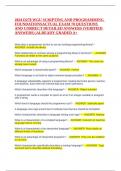
• Various point showing different E[rp] and p combinations providing equal utility to the investor
• How does the indifference curve of a less/more risk-averse investor compare to this indifference
curve?
Mean Variance Analysis
Which investor has a risk aversion coefficient equal to 4?
The higher level of U, the more risk averse someone is. Higher risk aversion index, higher the coefficient. 4 =
steeper line. X is risk y is return.
Basic Properties of Mean and Variance for Portfolio Returns
𝑅𝑃 = 𝑤1 𝑅1 + 𝑤2 𝑅2 + ⋯ + 𝑤1−𝑛 𝑅1−𝑛 + 𝑤𝑛 𝑅𝑛
𝐸[𝑅𝑃 ] = 𝑤1 𝜇1 + 𝑤2 𝜇2 + ⋯ + 𝑤1−𝑛 𝜇1−𝑛 + 𝑤𝑛 𝜇𝑛
3