Essay

ES2C5 - 1st - Wind Tunnel Lab Report - University of Warwick

1 purchase

Course
ES2C5 (ES2C5)

Institution
The University Of Warwick (UoW)

Lab Report for the Dynamics and Fluid Mechanics Module (ES2C5) as part of the Engineering Course at the University of Warwick which received a 1st (73%).

[Show more]

Preview 2 out of 5 pages

View example

Uploaded on July 30, 2024
Number of pages 5
Written in 2023/2024
Type Essay
Professor(s) Unknown
Grade A+

es2c5
dynamics
and
fluid
mechanics
lab
report
wind
tunnel
university
warwick
1st
engineering
mechanical
civil
electrical
1
21
22
3

Institution
The University of Warwick (UoW)
Education Unknown
Course
ES2C5 (ES2C5)

user2895729

Member since 2 year 30 documents sold

$9.89

Add to cart

Save

100% satisfaction guarantee
Immediately available after payment
Both online and in PDF
No strings attached

Wind Tunnel Lab
The main aim of this report is to investigate the complexity of fluid flow through 2 experiments.
For pressure distribution, 3 scenarios were investigated: full speed with mesh, full speed without
mesh, and half speed without mesh and the drag coefficient and separation angle was calculated.
When the boundary layer was laminar, Reynold’s number and the separation angle were shown
to be inversely proportional and when the boundary layer was turbulent, they were proportional.
For velocity distribution, 2 scenarios were considered: velocity of 10 𝑚𝑠 !" and 15 𝑚𝑠 !" however
two types of methods, were used to analyze the drag coefficients. In which, Reynold’s number
and the drag coefficient were found to be inversely proportional.

1. Introduction
The distinction between laminar and turbulent flow is an important concept in understanding the
behavior of fluid and fluid mechanics, since they are complex and have many real-life applications,
such as the aerodynamic analysis and shape optimization of a car. The aim of this report is to
investigate laminar and turbulent flow through experiments of pressure and velocity distributions
in relation to Reynold’s number, the drag coefficient, and the angle of separation.

2. Background Information
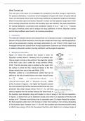
Figure 2.1 shows the potential flow around a circle, for
Reynold’s number below 5. However, this is not always true.
Take an object in a fluid, at the surface of the object the velocity
of the fluid is zero, this is called the no-slip condition (White,
Figure 2.2 - shows the pressure
2016). Then the boundary layer is defined as the region from Figuredistribu3on
2.1 - showsof poten3al
the streamﬂow around
pattern
of fluida flow
circleaccording
(White, 2016).
to different
the surface in which the flow velocity increases to the free- Reynold's number (Duranay, et al.,
stream velocity from zero at the wall (White, 2016). 2022).

Reynold’s number is a non-dimensional number that can be
defined as the ratio of inertial forces over shear viscous forces,
#$
𝑅𝑒 = %
where 𝑢 = 𝑐ℎ𝑎𝑟𝑎𝑐𝑡𝑒𝑟𝑖𝑠𝑖𝑡𝑐 𝑣𝑒𝑙𝑜𝑐𝑖𝑡𝑦, 𝐿=
𝑐ℎ𝑎𝑟𝑎𝑐𝑡𝑒𝑟𝑖𝑠𝑖𝑡𝑖𝑐 𝑙𝑒𝑛𝑔𝑡ℎ and 𝑣 = 𝑘𝑖𝑛𝑒𝑚𝑎𝑡𝑖𝑐 𝑣𝑖𝑠𝑐𝑜𝑠𝑖𝑡𝑦 (White,
2016). As shown in figure 2.1, the higher the Reynold’s number
the more turbulent the fluid flow because inertial forces are more
prominent than shear viscous forces. From 𝑅 = 9.6, the fluid Figure 2.2 - shows the pressure
distribution of potential flow around a
starts to separate from the surface because the shear forces in circle (White, 2016).
the boundary layer dissipate energy which leads to a loss of energy in the fluid and separation.
In figure 2.2, laminar flow can be explained visually since there is a separation of the fluid and
surface at 80°. Whereas inviscid theory has no separation point. For higher Reynold’s numbers,
the fluid separates earlier due to the increase in shear force leading to more energy dissipating
in the boundary layer. However, from 𝑅 = 500, 000 the boundary layer becomes turbulent which
in effect draws energy in from the free-stream fluid flow which leads to an increased angle of

1

, separation. Which, regarding figure 2.2, explains why the separation angle is 120° and the curve
rises after the minimum then levels off.
The drag coefficient is another non-dimensional number
which can be expressed as the drag force over dynamic
&
force, 𝐶& = ! where 𝐷 = 𝑑𝑟𝑎𝑔 𝑓𝑜𝑟𝑐𝑒, 𝜌 = 𝑑𝑒𝑛𝑠𝑖𝑡𝑦,
'#" (
"

and 𝐴 = 𝑎𝑟𝑒𝑎 (White, 2016). Figure 2.3 shows the
relationship between Reynold’s number and the drag
Figure 2.3 - shows the relationship between the
coefficient. For most values of Reynold’s number, the drag drag coefficient and Reynold’s number (White,
2016).
coefficient decreases as Reynold’s number increases.
In terms of calculations, pressure differences can be calculated using a multitube manometer,
using the equation ∆𝑝 = 𝜌𝑔ℎ (White, 2016). If there is one point where the pressure is known,
then we can calculate the other pressures using the measured height, known density, and
pressure as a comparison. We can increase the sensitivity of a multitube manometer by
increasing the angle of inclination. This is because small pressures will have larger effect along
the inclined length and leads to increased sensitivity and accuracy, ∆𝑝 = 𝜌𝑔𝑙𝑠𝑖𝑛𝜃 where 𝑙 =
𝑙𝑒𝑛𝑔𝑡ℎ, 𝑔 = 𝑔𝑟𝑎𝑣𝑖𝑡𝑎𝑡𝑖𝑜𝑛𝑎𝑙 𝑎𝑐𝑐𝑒𝑙𝑒𝑟𝑎𝑡𝑖𝑜𝑛 and 𝜃 = 𝑎𝑛𝑔𝑙𝑒 𝑜𝑓 𝑖𝑛𝑐𝑙𝑖𝑛𝑎𝑡𝑖𝑜𝑛. Moreover, the Bernoulli’s
'
principle can be used calculate the velocity by pressure differences, 𝑝 + 𝑢) + 𝜌𝑔ℎ = 𝑐𝑜𝑛𝑠𝑡
)
where ℎ = ℎ𝑒𝑖𝑔ℎ𝑡 (White, 2016). We can approximate definite integrals using the Trapezoidal and
Simpson’s rule. Trapezoidal rule uses linear approximations whereas, Simpson’s rule uses
quadratic approximation which makes it more accurate (Thangarajah, 2023). Therefore,
Simpson’s rule is more suited to a smooth function. The number of nodes indicates the points
used in the approximations; therefore, more nodes mean a larger accuracy.

3. Method
There will be 2 experiments conducted: pressure distribution and velocity distribution. For the first
experiment, a cylinder will have holes equally spaced by 15° from 0° till 180° which are attached
to plastic tubes which leads to a multitube manometer. There is also a pitot-static tube in free-
stream velocity to serve as a comparison. This cylinder is placed in a wind tunnel and the pressure
can be calculated. In the second experiment, using a pitot-static probe and moving it vertically to
measure velocity downstream of a cylinder. A micromanometer calculates the velocity using the
pressure difference between the pitot-static probe, static pressure and Bernoulli’s principle.

Figure 3.1 - shows the apparatus set up of the pressure distribution experiment and velocity distribution experiment respectively.

2

The benefits of buying summaries with Stuvia:

Guaranteed quality through customer reviews

Stuvia customers have reviewed more than 700,000 summaries. This how you know that you are buying the best documents.

Quick and easy check-out

You can quickly pay through credit card or Stuvia-credit for the summaries. There is no membership needed.

Focus on what matters

Your fellow students write the study notes themselves, which is why the documents are always reliable and up-to-date. This ensures you quickly get to the core!

Frequently asked questions

What do I get when I buy this document?

You get a PDF, available immediately after your purchase. The purchased document is accessible anytime, anywhere and indefinitely through your profile.

Satisfaction guarantee: how does it work?

Our satisfaction guarantee ensures that you always find a study document that suits you well. You fill out a form, and our customer service team takes care of the rest.

Who am I buying these notes from?

Stuvia is a marketplace, so you are not buying this document from us, but from seller user2895729. Stuvia facilitates payment to the seller.

Will I be stuck with a subscription?

No, you only buy these notes for $9.89. You're not tied to anything after your purchase.

Can Stuvia be trusted?

4.6 stars on Google & Trustpilot (+1000 reviews)

66902 documents were sold in the last 30 days

Founded in 2010, the go-to place to buy study notes for 15 years now

Start selling

Essay

ES2C5 - 1st - Wind Tunnel Lab Report - University of Warwick

Document information

Subjects

Written for

Seller

Reviews received

Content preview