100% satisfaction guarantee Immediately available after payment Both online and in PDF No strings attached
logo-home
MIS 180 EXCEL EXAM QUESTIONS AND ANSWERS ALL CORRECT $12.99   Add to cart

Exam (elaborations)

MIS 180 EXCEL EXAM QUESTIONS AND ANSWERS ALL CORRECT

 21 views  0 purchase
  • Course
  • MIS 180 EXCEL
  • Institution
  • MIS 180 EXCEL

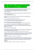
MIS 180 EXCEL EXAM QUESTIONS AND ANSWERS ALL CORRECT Place a dotted line border (the option directly under "None" in the "Border" tab of the "Format Cells" dialog window) under each subsequent row in the table. 1.1-1.5 - Answer-Home Tab> Highlight cells>Format> Format Cells>Border&gt...

[Show more]

Preview 2 out of 8  pages

  • August 29, 2024
  • 8
  • 2024/2025
  • Exam (elaborations)
  • Questions & answers
  • MIS 180 EXCEL
  • MIS 180 EXCEL
avatar-seller
Scholarsstudyguide
MIS 180 EXCEL EXAM QUESTIONS
AND ANSWERS ALL CORRECT
Place a dotted line border (the option directly under "None" in the "Border" tab of the
"Format Cells" dialog window) under each subsequent row in the table.
1.1-1.5 - Answer-Home Tab> Highlight cells>Format> Format Cells>Border>
"None">Dotted line

Fill rows 2 and 3 of the table (range B2:J3) using any color (not "No Fill") from the "Fill
Color" drop-down menu.
1.1-1.5 - Answer-Home tab>Fill icon

Set the print area of the worksheet to include only the area of the data table (Range
B2:J50)
1.1-1.5 - Answer-File>Highlight cells>Print Area

Set the left and right print margins of the worksheet to be .5 inches
1.1-1.5 - Answer-Page Layout> Print Margins> Custom Print

Set column B as "Columns to repeat at left" page titles
1.1-1.5 - Answer-File>Page Setup>Sheet>Highlight cells> Columns to repeat at left

In the same sort, first sort the table on the "World Records Sorted" worksheet by
Country in ascending order (A to Z) then sort the table by 'Record Date' in descending
order (Newest to Oldest).
32 8
11.12 - Answer-Hom Tab>Sort & Filter

Filter the table on the "World Records Sorted" worksheet to display only athletes whose
"Nationality" listed as "Kenya" or "Jamaica"
1.1-1.2 - Answer-Home Tab>Sort & Tab> Filter> Arrow should show up on cell

Construct a formula in cell D11 to calculate the sales tax amount for transaction 578. Be
sure to appropriately reference the transaction amount in cell C11 and the sales tax rate
in cell C8 so that your formula can be reused for the remaining transations.
21.25
FORMULAS - Answer-"=">"ref cell> "*">ref cell> enter

Construct a formula in cell E11 to calculate the total amount for transaction 578. Be sure
to appropriately reference the transaction amount in cell C11 and the sales tax amount
in cell D11 so that you can reuse your formula to calculate the total for the remaining
transactions.
21.25
FORMULAS - Answer-"=">"ref cell> "*">ref cell> "+"> ref cell> enter

, Use the SUM function to calculate the "Grand Total" in for all transactions in cell E24.
21.25
FORMULAS - Answer-"=Sum">"E11:E23"

Use the COUNT function to calculate the number of MLB teams in 1990 (range
G10:G39).
STATS
21.25 - Answer-Formulas> insert function> count

Use the COUNTA function to calculate the number of MLB teams in 2010 (use range
F10:F39).
STATS
21.25 - Answer-Formulas>Insert function> COunta

Use the SUM function to calculate the total amount of salaries paid in 1990.
STATS
21.25 - Answer-Formulas>Insert Function>SUM

Use the AVERAGE function to calculate the average salary for the teams in 1990.
21.25
STATS - Answer-Formulas> Insert Function> AVERAGE

Use the MAX function to determine the maximum team salary amount in 1990.
21.25
STATS - Answer-Formulas>Insert Function>MAX

Use the MIN function to determine the minimum team salary amount in 2010.
2125
STATS - Answer-Formulas>Insert Function>MIN

Insert a new column between columns B and C. Label the new column (cell C3)
"Record ID" 1.1-1.5 - Answer-Home tab>Insert green button>insert column or row sheet

Use the "Fill" feature of Excel to insert the numbers 1 to 47 in cells C4:C50. 1.1-1.5 -
Answer-Type #1, #2> Home tab> Blue down arrow> Series> Autofill

Make the table headers (range B3:J3) bold 1.1-1.5 - Answer-Home tab>Bolded B

Center the table headers (range B3:J3) horizontally 1.1-1.5 - Answer-Home tab>
Highlight cells> Middle lines

Merge and center cell G2 across columns G:J
1.1-1.5 - Answer-Home Tab> Right button with lines/blue arrow> Merge & Center

Change the format of the date range (G4:G73) to "Short Date"

The benefits of buying summaries with Stuvia:

Guaranteed quality through customer reviews

Guaranteed quality through customer reviews

Stuvia customers have reviewed more than 700,000 summaries. This how you know that you are buying the best documents.

Quick and easy check-out

Quick and easy check-out

You can quickly pay through credit card or Stuvia-credit for the summaries. There is no membership needed.

Focus on what matters

Focus on what matters

Your fellow students write the study notes themselves, which is why the documents are always reliable and up-to-date. This ensures you quickly get to the core!

Frequently asked questions

What do I get when I buy this document?

You get a PDF, available immediately after your purchase. The purchased document is accessible anytime, anywhere and indefinitely through your profile.

Satisfaction guarantee: how does it work?

Our satisfaction guarantee ensures that you always find a study document that suits you well. You fill out a form, and our customer service team takes care of the rest.

Who am I buying these notes from?

Stuvia is a marketplace, so you are not buying this document from us, but from seller Scholarsstudyguide. Stuvia facilitates payment to the seller.

Will I be stuck with a subscription?

No, you only buy these notes for $12.99. You're not tied to anything after your purchase.

Can Stuvia be trusted?

4.6 stars on Google & Trustpilot (+1000 reviews)

79271 documents were sold in the last 30 days

Founded in 2010, the go-to place to buy study notes for 14 years now

Start selling
$12.99
  • (0)
  Add to cart