100% satisfaction guarantee Immediately available after payment Both online and in PDF No strings attached
logo-home
BA 325 Practice Detailed Answer Test 2024/2025 $14.99   Add to cart

Exam (elaborations)

BA 325 Practice Detailed Answer Test 2024/2025

 2 views  0 purchase

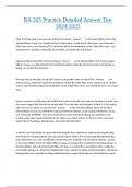
Filter the State column so only rows with MD are shown. Answer: In the Home Ribbon Tab in the Editing Ribbon Group, you clicked the Sort & Filter button. In the Sort & Filter menu, you clicked the Filter menu item. You clicked cell D1, clicked the Quick Sort dropdown. In the Table Filter me...

[Show more]
Preview 3 out of 22  pages

  • August 30, 2024
  • 22
  • 2024/2025
  • Exam (elaborations)
  • Questions & answers
All documents for this subject (7)
avatar-seller
Schoolflix
BA 325 Practice Detailed Answer Test
2024/2025

Filter the State column so only rows with MD are shown. Answer: In the Home Ribbon Tab in the
Editing Ribbon Group, you clicked the Sort & Filter button. In the Sort & Filter menu, you clicked the
Filter menu item. You clicked cell D1, clicked the Quick Sort dropdown. In the Table Filter menu, you
clicked the VA checkbox, clicked the DE checkbox, and clicked the OK button.


Apply workbook protection to this workbook. Answer: In the Review Ribbon Tab in the Changes
Ribbon Group, you clicked the Protect Workbook button. Inside the Protect Structure and Windows
dialog, you clicked the OK button.


Sort this data by the Date of Last Visit column so the oldest dates are listed first. Answer: You
clicked cell G1, clicked the Quick Sort dropdown, clicked the Table Filter menu, clicked cell G2, clicked
cell G1, and clicked the Quick Sort dropdown. In the Table Filter menu, you clicked the Sort A to Z menu
item.


Enter a formula in cell B2 using the VLOOKUP function to find the total sales for the date in cell B1. Use
the named range DailySales for the lookup table. The total sales are located in column 5 of the lookup
table. Be sure to require an exact match. Answer: In the Formulas Ribbon Tab in the Function
Library Ribbon Group, you clicked the Lookup & Reference button. In the Lookup & Reference menu,
you clicked the VLOOKUP menu item. Inside the Function Arguments dialog, you typed B1 in the
Lookup_value input, typed DailySales in the Table_array input, typed 5 in the Col_index_num input,
typed False in the Range_lookup input, and clicked the OK button.


In cell A2, use Consolidate to create subtotals using the Sum function for values in the named range
ItemsOrdered. Include both the top row and left column labels. The named range ItemsOrdered has
been defined for you. The consolidation should show the subtotals only and not the details. Answer:
In the Home Ribbon Tab in the Styles Ribbon Group, you clicked the Conditional Formatting button. In
the Data Ribbon Tab in the Data Tools Ribbon Group, you clicked the Consolidate button. Inside the
Consolidate dialog, you clicked the DialogHeader view, clicked the dialog undefined button, clicked the
DialogHeader view, clicked the dialog undefined button, typed ItemsOrdered in the Reference input,

,clicked the All references list, checked the Top row check box, checked the Left Column check box, and
clicked the OK button.


On the Summary sheet, in cell B3, enter a formula to display the value of cell B3 from the ByMonth
sheet. Answer: You clicked cell B3, typed = in cell B3, clicked the ByMonth tab, clicked the Summary
tab, clicked cell B3, clicked the formula bar, typed "=ByMonth!Summary!B" in the formula bar, clicked
the formula bar, typed "=" in the formula bar, clicked the ByMonth tab, clicked cell B3, and pressed
Enter.


Apply conditional formatting to the selected cells so cells with a value greater than 10 are formatted
using a yellow fill with dark yellow text. Answer: In the Home Ribbon Tab in the Styles Ribbon
Group, you clicked the Conditional Formatting button. In the Conditional Formatting menu in the
Highlight Cells Rules menu, you clicked the Greater Than... menu item. Inside the Greater Than dialog,
you typed 10 in the Format cells that are GREATER THAN: input. Inside the Greater Than dialog in the
with drop-down, you selected Yellow Fill with Dark Yellow Text. Inside the Greater Than dialog, you
clicked the OK button.


Insert a clustered column-line combination chart based on the selected data. The line chart should
represent the Total Sales data series. Both data series should be on the primary axis. This is the first
chart type in the Combo Chart gallery. Answer: In the Insert Ribbon Tab in the Charts Ribbon Group,
you clicked the Insert Column or Bar Chart button. You selected the cell range A1:D3. In the Insert
Ribbon Tab in the Charts Ribbon Group, you clicked the Insert Combo Chart button. In the Insert Combo
Chart menu, you selected the Clustered Column - Line option.


Apply the Top and Double Bottom Border to the selected cells with a single command. Answer: In
the Home Ribbon Tab in the Font Ribbon Group, you clicked the Borders button arrow. In the Borders
menu, you clicked the Top and Double Bottom Border menu item.


Enter a formula in cell E2 using AVERAGEIFS to calculate the average price (use the named range
JunePrices) where the value in the JunePOs named range is equal to the value in cell D1 and the value in
the JuneCompanies named range is equal to the text string "DermoMagic". Answer: In the Formulas
Ribbon Tab in the Function Library Ribbon Group, you clicked the More Functions button. In the More
Functions menu in the Statistical menu, you clicked the AVERAGEIFS menu item. Inside the Function
Arguments dialog, you typed JunePrices in the Average_range input, typed JunePOs in the

, Criteria_range1 input, typed D1 in the Criteria1 input, typed JuneCompanies in the Criteria_range2
input, typed DermoMagic in the Criteria2 input, and clicked the OK button.


Enter a formula in cell C3 using the SUMPRODUCT function to calculate the total income by multiplying
the daily special price by the number of daily sales. Use the range names SpecialPrice and
MembershipsSold. Answer: In the Formulas Ribbon Tab in the Function Library Ribbon Group, you
clicked the More Functions button, clicked the Math & Trig button. In the Math & Trig menu, you clicked
the SUMPRODUCT menu item. Inside the Function Arguments dialog, you typed SpecialPrice in the
Array1 input, typed MembershipsSold in the Array2 input, and clicked the OK button.

History


Display the data table, including the legend keys. Answer: In the Design Ribbon Tab in the Chart
Layouts Ribbon Group, you clicked the Add Chart Element button. In the Add Chart Element menu in the
Data Table menu, you selected the Chart Elements Data Table With Legend Keys option.


Insert a recommended PivotTable, using the Sum of Total Spent by State option. Answer: In the
Insert Ribbon Tab in the Tables Ribbon Group, you clicked the PivotTable button. Inside the Create
PivotTable dialog, you clicked the Cancel button. In the Insert Ribbon Tab in the Tables Ribbon Group,
you clicked the Recommended PivotTables button. Inside the Recommended PivotTables dialog, you
clicked the OK button.


Use AutoFill to copy the formula and formatting in cell B9 to cells C9:D9. Answer: You pressed the
Ctrl + C keyboard shortcut, selected the cell range C9:D9, and pressed the Ctrl + V keyboard shortcut.


Add slicers to filter the data in this table by City. Answer: In the Design Ribbon Tab in the Tools
Ribbon Group, you clicked the Insert Slicer button. Inside the Insert Slicer dialog, you checked the City
check box, clicked the OK button.


Rename Sheet1: PO Q3. Answer: You double-clicked the Sheet1 tab, typed "PO Q3", and pressed
Enter.

The benefits of buying summaries with Stuvia:

Guaranteed quality through customer reviews

Guaranteed quality through customer reviews

Stuvia customers have reviewed more than 700,000 summaries. This how you know that you are buying the best documents.

Quick and easy check-out

Quick and easy check-out

You can quickly pay through credit card or Stuvia-credit for the summaries. There is no membership needed.

Focus on what matters

Focus on what matters

Your fellow students write the study notes themselves, which is why the documents are always reliable and up-to-date. This ensures you quickly get to the core!

Frequently asked questions

What do I get when I buy this document?

You get a PDF, available immediately after your purchase. The purchased document is accessible anytime, anywhere and indefinitely through your profile.

Satisfaction guarantee: how does it work?

Our satisfaction guarantee ensures that you always find a study document that suits you well. You fill out a form, and our customer service team takes care of the rest.

Who am I buying these notes from?

Stuvia is a marketplace, so you are not buying this document from us, but from seller Schoolflix. Stuvia facilitates payment to the seller.

Will I be stuck with a subscription?

No, you only buy these notes for $14.99. You're not tied to anything after your purchase.

Can Stuvia be trusted?

4.6 stars on Google & Trustpilot (+1000 reviews)

73216 documents were sold in the last 30 days

Founded in 2010, the go-to place to buy study notes for 14 years now

Start selling
$14.99
  • (0)
  Add to cart