Advanced Ecomometrics
Herhaling linear models
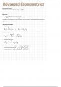
Remember the standard regression model y
=
XB + E
Conditioning
7
Conditioning is important in econometrics
2
VB what is variance today, given yesterday
Remember that an assumption of the classic linear regression model is that should be fixed therefore we
condition on
Some important formulas
·
Marginal density
f(y) =
JA(x y)dx
,
or f(x) =
(f(x y)dy ,
·
Conditional density
b(y x)f(y x)
, ,
f(yx) =
f(x) Sh(y x) by=
,
⑧
Conditional expectation
Elyx] =
Syb(y(x) dy
·
Conditional variance [y(x] E[(y ETy(x])"(x]
·
var : -
·
Law of iterated expectations E[y] Ex[Eyix [y(x]]
· :
·
Marginal variance :
(y) E[var (y(x)]
var =
(E[y(x]) + var
,Regressions and loss functions
Remember that the residuals are e =
y
-
y
7
Predictor : =
Xb Expected loss:
2
Real value :
y
=
XB + E
E[L(y y)() -
& We have different loss functions L(e) =
((y -y)
E[y(x]
2
8 :
8
Squared error .
e
y
①
Absolute error let :
Y =
med(y(x)
(1 x) if
E
-
e eso
8
Asymptotic absolute error ~
X e
if ezo
j =
q(y(x)
&
Step loss ·
Cite e-O
y =
mod(y(x)
The goal is to minimize the error, therefore we need an optimal predictor
to minimize the error. Every loss function has an optimal predictor.
Linear prediction
Ordinary least squares: goal again to minimize errors =
minei) mine-min -
(yiyi)
3
Y
I
XB xie ..
·)
xik
E[nX]
·
Yo · x
:
,
P =
: :
:
I :
xine
i
Yo
·
Xn2
...
Bu
OLS estimator minimizes - (yi -xib)2 =
ni =
(y XB)'(y XB)
-
-
boe-2Xy 2XX
=
+ 0
Bas (XX)"Xig - is the estimator of B
, -Y
P X(XX)"X'
n Matrix P projects Y on S(x)
:
e =
My M 1 P
and matrix M projects Y on So(x)
= -
D
I
> S(x) S
Both symmetric
y =
Xb =
Py and indempotent
Assumptions OLS
I
Fixed regressors: all elements of matrix X are fixed/non-stochastic rank (X) : :
b
2
Random disturbances Elui] : =
o
3
Homoskedasticity (disturbances have constant variance) Var (vi) z In : : =
4
No correlation between disturbances Cov (vi uj) ·
,
= o
5
Constant parameters B constant ·
6
Linear relation y XB : = +
u
uX N(0 In)
7
Normality: is normally distributed
E : -
,
X
Under these assumptions we have:
Unbiased: Variance:
E(B(X) B (XX)XEZuIX B : + =
BLUE:
v(B(x) j(XX)" = -
any other estimator Distribution:
b(X -
N(B , (XX)")
N
Asymptotic theory
T
In asymptotic theory the assumption of normality is dropped, however we can still get the same result
by R -D
We first repeat some theories
8
i.i.d: independent and identically distributed
O
i.n.i.d: independent and not identically distributed
Modes of convergence
3
O
Converges in distribution Xn° X if im Fr(x) : -
F(x)) = o
O
Converges in probability Xn"-X plimXn X if :
or
= im PXn-X1 > = Yn **
X = > Xn
:
/
Converges almost surely Xn Xif P in /Xn-X1 Xn X
M S
O ** .
..
:
X
=
0 =
8
Converges in mean square XnXif nhmE (Xn-X)2 : =
, Law of Large Numbers
-n-gr -8
&
Weak (WLLN): in probability
&
Strong (SLLN): almost surely
e
Khintchine WLLN EXiBis id Mi ·
,
=
pe
O
Chebyshev WLLN :
[XiDiz him =
, ind
O
Markov SLLN EXi ·
is ,
indo
Central Limit Theorem
Zi
M -Wo , we
&
Lindeberg-Levy CLT EXiSiz id Mi p i 82 ·
,
inid
= =
Lindeberg-Feller CLT [Xibic hi E (Xi-mi(Xi mis)]
6 ·
, =
)
Liapounov CLT [Xi inid him (2 Ei
+
O ·
is ,
Transformation theory
If Xn X and Yn se If Xn"X and An " A
·
Xn + Yn X + e
·
AnXn AX
·
XnYn eX · An"Xn"A"X
·
Xn/Yn -
X/e
Delta method
·
·
n
~N(A n20)
(g(fn)
,
-
g(fo))d
g(n)
N(o
-
,
N(g(f)
nGe)]G(8)
Gi) Goe .
,
:
ag(t)
at
2
Instead of the normality assumption we assume that n is large and add new assumptions
⑧
Stability of X
plim ( * XX) plim (n Exixi') Mxx
= =
⑧
Orthogonality of X and u
plim (Xa) = o
&
Stability of u
plim (in'u) = and
plines" =
N
Using these assumptions we have
The benefits of buying summaries with Stuvia:
Guaranteed quality through customer reviews
Stuvia customers have reviewed more than 700,000 summaries. This how you know that you are buying the best documents.
Quick and easy check-out
You can quickly pay through credit card or Stuvia-credit for the summaries. There is no membership needed.
Focus on what matters
Your fellow students write the study notes themselves, which is why the documents are always reliable and up-to-date. This ensures you quickly get to the core!
Frequently asked questions
What do I get when I buy this document?
You get a PDF, available immediately after your purchase. The purchased document is accessible anytime, anywhere and indefinitely through your profile.
Satisfaction guarantee: how does it work?
Our satisfaction guarantee ensures that you always find a study document that suits you well. You fill out a form, and our customer service team takes care of the rest.
Who am I buying these notes from?
Stuvia is a marketplace, so you are not buying this document from us, but from seller maaikekoens. Stuvia facilitates payment to the seller.
Will I be stuck with a subscription?
No, you only buy these notes for $6.96. You're not tied to anything after your purchase.