Univariate linear time series
Time serie is a sequential set of observations on variable x, where t represents time Exa =..., Xe-2 ,
Xe ,
Xe ,
Xe +, Xe +, ...
Financial returns
-
One-period (simple) return PA Pe DA Pt-1 Pt Pt-1 DE
note
PA
-
+
-
- - 1
regular (if dividends are included
: RE =
Pt-1 Rt =
Pt -1 =
Pe -
1
+
Pt -1
) RE
returns
log-return =log) Rt) leg (p) :
log -log Pr , +
= =
pr -pe
= Pr =
spe Pt
price
-
Multi-period return (sum of one-period returns), use log-returns k - 1
dividens
De
re[k] =
pt
-
pe m
=
(pt -
pt
1) -
(pt ps k)
- =
ra +
(pt 1
-
pe
-z) +
(pec -
pe
-b) =
ra + re + ...
grej
#
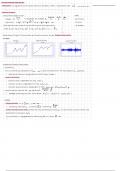
Using these concepts of time series and financial returns, we get financial time series
example
Prices Log of prices Log of return
properties financial time series
-
stationarity
strict stationarity: distribution of (xh + 1,
, . . .,
Xer +
1) does not depend on t for any integers Et , ....
Ab and t
distribution does not change when we shift, hence change t
7
weak stationarity
8
constant mean, independent of time: E(xt) M =
O
constant variance, independent of time: Var(xe) G =
El(x m)(x )]
constant autocovariance, independent of time: (x
e)
O
for( j
: - -
=
,
-
autocorrelation function ACF: pl =
core (xt ,
xx e) =
Var(xe) =
yo
D E(ae) Var(ae) Cov(at are)
example stationary process, White Noise: = 0
,
=
8, ,
=
o
models
d
Linear process: m j +jatj m Xt =
+ = + Nodt + 4 , at - ....
Pit
stationary with mean M , variance z4, and ACF Al 204j
7 =
Wold's decomposition theory states that any stationary proces [xe] can be written as sum of linear and
deterministic processes Ewa]
We could also at a lag operator B, defined by Bxt =
XA -
, hence Baxt =
Xe b -
I
, N
Then we could write the linear process as xt =
m
+ x(B) at =
m
+ 4oat + 4 , at - ...
+ That - b
- +(B) =
j4 B ,
8
Autoregressive process
· AR( ) ,
:
xt =
00 + Ext -1 + at
①o Ga
7
stationary if 10 14 , then E(x) A Var(xz) -0 ,
yo
= =
m
=
. =
1 -
, 1
proof 00 Xt = + 6 , Xt -
1 + at
(1 -
d, B) xt =
00 + at
x =
,)1 qB)" (d at)
-
+ =
j(q B)" (4,
+ a) =
Tod, (0 +
atj)
-
d(B) =
1 - d B ,
=
0
&
AR( ) 4
5
ACF ,
stationary 1
is linear process with exponentially decaying weights =
6 ,
, we find =
pe
=
0
AR(p)
·
:
xt = do + d , xt -
1 + +
6pxt -
p
+ at
example
...
Et
ye
0
3yt +
=
0
1yt
. - + .
-
2
>
stationary if all zj lie outside unit circle: ye
-
0 .
3yt -
1
-
0 .
1yt 2
=
Et
xt- t
proof X- ·
,
(1 -
0 .
3) -
o .,
(2) ye =
Es
↓ (2) 122
for =
1 -
0 32.
-
0 .
= 0 2 = -
522 = 2
((z) =
1 -
0 , 2 ....
-
pzP = 0 #
as both lie outside unit circle, stationary
&
ACF can not be determined, but we can use partial autocorrelation function (PACF), for
AR(p), the PACF has cut-off point at l p =
Q
Moving Average model
·
MA(1) :
x =
20 + at -
G at -1
,
7
stationary for all parameter values with M ja) +i)
jo er =
=
1 +
,
-- for hence ACF is cut-off at l peo
>
,
p 1
. =
,
>
invertible if 18 14 .
, a model is invertible if it can be expressed as AR(n)
proof XA =
at + fat -
1
at =
xx
-
G , at -
1
=
Xt - 0(xt - - at z) =... =
x -
Ext + + 0xx 2 - 83x 3 + ...
D
( f)" AR(g) 101
= -
i =
-
+ a =
only works as
>
PACF decays exponentially
MA(q)
·
at-Gat- . . .
xt co
gatg
-
: = +
>
ACF has cut-off point at l g =
invertible if all roots zj lie outside unit circle: Fiat -
at
gatq
7
Xt e0
-
=
+ -
-...
xe =
e +
1) -
f B ,
-
...
fqB) at ,
Xe = e + (B) at
6(z) =
1
-
12 ...
-
gz = o
&
PACF decays exponentially
, &
Mixed autoregressive-moving average model
ARMA(p g)
·
d dx ApX - G,
,
EqAq :
xt = + + + ... +
-p
+ at ....
①o O(z)
b(z) y(B)at (2)
stationary if all roots of
7
lie outside unit circle, implying xx =
m
+
,
m
=
0)) ,
=
q(z)
((z)
3
invertible if all roots of f(z) lie outside unit circle, yielding # (B) x1 = co + at
,
20 =
0(1) ,
(2) =
f(z)
7
ACF decays exponentially
>
PACF decays exponentially
&
ARMA(p 1)
To avoid identification problems, reduce model to -1 ,
g
-
Stuvia customers have reviewed more than 700,000 summaries. This how you know that you are buying the best documents.
Quick and easy check-out
You can quickly pay through credit card or Stuvia-credit for the summaries. There is no membership needed.
Focus on what matters
Your fellow students write the study notes themselves, which is why the documents are always reliable and up-to-date. This ensures you quickly get to the core!
Frequently asked questions
What do I get when I buy this document?
You get a PDF, available immediately after your purchase. The purchased document is accessible anytime, anywhere and indefinitely through your profile.
Satisfaction guarantee: how does it work?
Our satisfaction guarantee ensures that you always find a study document that suits you well. You fill out a form, and our customer service team takes care of the rest.
Who am I buying these notes from?
Stuvia is a marketplace, so you are not buying this document from us, but from seller maaikekoens. Stuvia facilitates payment to the seller.
Will I be stuck with a subscription?
No, you only buy these notes for $7.02. You're not tied to anything after your purchase.