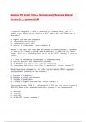
This summary concerns the subject of quantitative research methodology and is written on the basis of the book by Andy Field. The summary also deals with the methods used by SPSS and how tables should be read.
Chapter 2 THE SPINE OF STATISTICS
Chapter 2.2 What is the SPINE of statistics?
You should focus on the similarities between statistical models rather than the
differences. The mathematical form of the model changes, but it usually boils down to a
representation of the relations between an outcome and one or more predictors. If you
understand this, there are five key concepts; the SPINE of statistics:
- Standard error
- Parameters
- Interval estimates (confidence intervals)
- Null hypothesis significance testing
- Estimation
Chapter 2.3 Statistical models
A model can be used to predict things about the real world. Therefore, it is important that
the model accurately represents the real world. In research: the statistical model should
represent the data collected (the observed data) as closely as possible. The degree to
which there is a match is called the fit of the model.
Everything in this book (and statistics in general) boils down to: outcome i= ( model ) +error i
- This means that the data we observe can be predicted from the model we choose
to fit plus some amount of error.
- The ‘i’ refers to the ‘ith’ score; the value and outcome are different for each score.
Chapter 2.4 Populations and samples
A population can be very general or very narrow. Scientist are interested in the general.
“We rarely, if ever, have access to every member of a population. Psychologists cannot
collect data from every human being. Therefore, we collect data from a smaller subset of
the population known as the sample and use these data to infer things about the
population as a whole.”
- The bigger the sample, the more likely it is to reflect the entire population.
Chapter 2.5 P is for parameters
Statistical models are made up of variables and parameters.
- Variables: measured constructs that vary across entities in the sample.
- Parameters: not measured and are (usually) constant believed to represent some
fundamental truth about the relations between variables in the model (e.g. mean
and median).
When we are interested in predicting an outcome using only a parameter, we use the
following equation.
- outcome i =( b 0 ) +error i
Often, we want to predict an outcome from a variable, and if we do this, we expand the
model to include this variable (predictor variables are usually denoted with the letter ‘X’).
Our model becomes:
- outcome i =( b 0 +b1 X i ) +error i
In this case we are predicting the value of the outcome for a particular entity (i) not just
from the value of the outcome when there are no predictors (b 0) but from the entity’s
score on the predictor variable (Xi). the predictor variable has a parameter (b1) attached
to it, which tells us something about the relationship between the predictor and the
outcome. If we want to predict an outcome from two predictors then we can add another
predictor to the model:
- outcome i =( b 0 +b1 X 1 i + b2 X 2 i ) +error i
In this model we are predicting the value of the outcome for a particular entity (i) from
the value of the outcome when there are no predictors (b0) and the entity’s score on two
predictors (X1i and X2i). each predictor variable has a parameter (b1 and b2) attached to it.
To work out what the above models look like, we estimate the parameters (i.e., the
value(s) of b).
1
,The reason being is that we don’t know what the parameter values are in the population
because we didn’t measure the entire population, we measured only a sample. We can
use the sample to make an estimate (which is why the word ‘estimate’ is used).
The mean-value is a hypothetical value: it is a model created to summarize the data and
there will be error in prediction. When you see equations where ‘hats’ (^) are used, this
will make explicit that the values underneath them are estimates.
It is important to assess the fit of any statistical model. This can be done by comparing
the predicted scores with the actual values as observed in the data.
- The error (:) is calculated by subtracting the predicted score from the actual
observed score. It is also called the deviance.
o Deviance=outcome i−model i
o A negative ‘error-number’ shows that the model overestimates.
To calculate the overall error of the model we should use another equation. We can’t add
all the separate deviances (or: errors) because the total would be zero. The only way
around this, is to square the errors. This will give the following equation:
- ∑ of squared errors ( SS )=¿
o This equation looks similar to: of squares=¿
∑
When talking about models in general, the following equation is best suited:
- Total error=¿
o This model can be used to assess the total error in any model
The sum of squared error (SS) is a good measure of the accuracy of our model. However,
it depends upon the quantity of data that has been collected (the more data points, the
higher the SS). To overcome this, we can use the average error, rather than the total.
- Average error: the sum of squares (i.e. total error) by the number of values (N)
that we used to compute that goal.
- To estimate the mean error in the population we need to divide not by the
number of scores contributing to the total, but by the degrees of freedom (df),
which is the number of scores used to compute the total adjusted for the fact that
we are trying to estimate the population value.
SS
o Mean squared error= =¿ ¿
df
The sum of squared error and the mean of squared error (variance) can be used to
assess the fit of a model.
- Large values relative to the model indicate a lack of fit.
Chapter 2.6 E is for estimating parameters
This section has focused on the principle of minimizing the sum of squared errors, and
this is known as the method of least squares of ordinary least squares OLS.
Chapter 2.7 S is for standard error
Sample variation: when the mean of a sample is different than the mean of a different
sample (within the same population). Samples vary because they contain different
members of the population.
Sampling distribution: a histogram which shows the results of the different samples
taken. Frequency distribution of sample means (or whatever parameter you’re trying to
estimate).
An average of all sample means would give us the population mean.
- Bearing in mind that the average of the sample means is the same as the
population mean, the standard deviation of the sample means would therefore tell
us how widely sample means are spread around the population mean: put
another way, it tells us whether sample means are typically representative of the
population mean.
2
,Standard error of the mean (or: standard error) (SE): the standard deviation of sample
means. This can be calculated by taking the difference between each sample mean and
the overall mean, squaring these differences, adding them up, and then dividing by the
number of samples. Finally, the square root of this value would need to be taken to get
the standard deviation of sample means: the standard error.
Central limit theorem: samples get large (usually defined as greater than 30), the
sampling distribution has a normal distribution with a mean equal to the population
mean, and a standard deviation shown in equation:
s
- σ x̄ =
√N
Chapter 2.8 I is for (confidence) interval
Confidence interval: the boundaries within which we believe the population value will fall.
Point estimate: a single value from the sample.
Interval estimate: using our sample value as the midpoint, but set a lower and upper limit
as well.
The crucial thing is to construct the intervals in such a way that they tell us something
useful. For example, perhaps we might want to know how often, in the long run, an
interval contains the true value of the parameter we are trying to estimate. This is what a
confidence interval does. Typically, we look at 95% confidence intervals, and sometimes
99% confidence intervals, but they all have a similar interpretation.
- Confidence interval: they are limits constructed such that, for a certain
percentage of samples (be that 95% or 99%), the true value of the population
parameter falls within the limits.
o The trouble is, you don’t know whether the confidence interval from a
particular sample is one of the 95% that contain the true value or one of
the 5% that do not.
To calculate the confidence interval, we need to know the limits (boundaries) within
which 95% of sample means will fall. The 1.96 is the z-score relevant to a 95%
confidence interval.
- lower boundary of confidence interval= x̄ − ( 1.96∗SE )
- upper boundary of confidence interval= x̄ + ( 1.96∗SE )
Calculating confidence intervals in large samples (using z-scores):
If a confidence interval is very wide then the sample mean could be very different from
the true mean, indicating that it is a bad representation of the population (and the other
way around).
In general, we can say that confidence intervals of proportions are calculated as follows.
lower boundary of confidence interval= x̄ − z 1−p ∗SE
- ( 2
)
upper boundary of confidence interval= x̄ + z ∗SE
- ( 1− p
2
)
The procedure mentioned above is fine for large samples, since the central limit theorem
tells us that the distribution will be normal. However, for small samples, the sampling
distribution is not normal – it has a t-distribution.
Calculating confidence intervals in small samples (using t-values):
T-distribution: a family of probability distributions that change shape as the sample size
gets bigger (when the sample size gets very big, it has the shape of a normal
distribution).
3
, - lower boundary of confidence interval= x̄ −( t n−1∗SE )
- upper boundary of confidence interval= x̄ + ( t n−1∗SE )
When looking up a z-score, you should figure out if it contains the larger part of the
normal distribution (body) or the smaller part (tail). The larger portion refers to the larger
part of the graph (aka the body), the smaller portion refers to the smaller part of the
graph (aka the tail).
- Body means looking at the values stated under ‘larger portion’.
- Tail means looking at the values stated under ‘smaller portion’.
Figure: Body and tail (equals: ‘larger portion’ and ‘smaller portion’)
A confidence interval is usually displayed using an error bar, see figure below.
Figure: Confidence interval (error bar)
The confidence interval tells us the limits within which the population mean is likely to
fall.
- By comparing the confidence intervals of different means (or other parameters)
we can get some idea about whether the means came from the same or different
populations. (We can’t be entirely sure because we don’t know whether our
particular confidence intervals are ones that contain the population value or not.)
- When confidence intervals (the ranges) don’t overlap at all, there are two
possibilities:
o Our confidence intervals both contain the population mean, but they come
from different populations (and therefore, so do our samples)
o Both samples come from the same population but one (or both) of the
confidence intervals doesn’t contain the sample mean (because in 5% of
the cases, they don’t (95% confidence)).
This is why error bars are useful: because if the bars of any two means do not overlap (or
overlap only by a small amount) then we can infer that these means are from different
populations – they are significantly different.
Chapter 2.9 N is for null hypothesis significance testing
NHST: null hypothesis significance testing
Alternative hypothesis (H1) (or: experimental hypothesis): the hypothesis or prediction
from your theory would normally be that an effect will be present.
4
The benefits of buying summaries with Stuvia:
Guaranteed quality through customer reviews
Stuvia customers have reviewed more than 700,000 summaries. This how you know that you are buying the best documents.
Quick and easy check-out
You can quickly pay through credit card or Stuvia-credit for the summaries. There is no membership needed.
Focus on what matters
Your fellow students write the study notes themselves, which is why the documents are always reliable and up-to-date. This ensures you quickly get to the core!
Frequently asked questions
What do I get when I buy this document?
You get a PDF, available immediately after your purchase. The purchased document is accessible anytime, anywhere and indefinitely through your profile.
Satisfaction guarantee: how does it work?
Our satisfaction guarantee ensures that you always find a study document that suits you well. You fill out a form, and our customer service team takes care of the rest.
Who am I buying these notes from?
Stuvia is a marketplace, so you are not buying this document from us, but from seller jaccoverbij. Stuvia facilitates payment to the seller.
Will I be stuck with a subscription?
No, you only buy these notes for $3.20. You're not tied to anything after your purchase.