100% satisfaction guarantee Immediately available after payment Both online and in PDF No strings attached
logo-home
Data Structures (2IL50) Summary 2020 $4.34   Add to cart

Summary

Data Structures (2IL50) Summary 2020

1 review
 406 views  3 purchases
  • Course
  • Institution

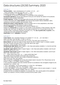
EN: Data Structures (2IL50) is a course given at Eindhoven University of Technology. It is a mandatory course for Bachelor Computer Science and Engineering students. It is given in the third quartile of the first year. Data structures delves deeper into the content discussed in Discrete Structures ...

[Show more]
Preview 2 out of 8  pages

  • May 28, 2020
  • 8
  • 2019/2020
  • Summary

1  review

review-writer-avatar

By: cminhphm • 3 year ago

avatar-seller
Data structures (2IL50) Summary 2020
Lecture 1
Sorting problem: - input: array/sequence of n number < a1, a2, …, an >
- output: permutation of the input such that < ai1 ≤ … ≤ ain >
A complete description of an algorithm consists of 3 parts:
1) The algorithm 2) The proof of correctness 3) The derivation of the running time
Incremental algorithms: process input elements one-by-one and maintain the solution for the elements
processed so far. Example: InsertionSort
In place algorithm: numbers are rearranged within the array with only constant extra space.
To prove correctness with a loop invariant, show that the loop invariant holds at initialization (start),
maintenance (during the program) and termination (finish).
Divide-and-conquer sorting algorithm: break the problem into 2 or more subproblems, solve these
recursively and combine these solutions to give an answer.
Example: MergeSort. The correctness proof is done by induction on n.
Analyze the running time as a function of n (the number of input elements) in these situations: best case,
average case, worst case. An algorithm has worst case running time T(n) if for any input of size n the
maximal number of elementary operations executed is T(n). The rate of growth/order of growth of the
running time is far more important than constants.
InsertionSort: Θ(n^2). MergeSort: Θ(nlog(n))

Lecture 2
Linear Search: input: increasing sequence of n numbers A = < a1, a2, …, an > and value v
output: and index i such that A[i] = v or NIL if v not in A.
This is done from start to end of the array until v is found. Thus worst case running time: n
Binary Search: see input and output of Linear Search. But here it checks if value v is smaller or greater
than value at pointer and goes to half of correct side. Worst case: log(n).
Let g(n): N -> N be a function. Then we have:
Asymptotically tight bound (equal): Θ(g(n)) = { f(n): there exist positive constants c1, c2 and n0 such that
c1 * g(n) ≤ f(n) ≤ c2 * g(n) for all n ≥ n0 }
Asymptotic upper bound (smaller or equal): Ο(g(n)) = { f(n): there exist positive constants c and n0 such
that f(n) ≤ c*g(n) for all n ≥ n0 }
Asymptotic lower bound (greater or equal): Ω(g(n)) = { f(n): there exist positive constants c and n0 such
that c * g(n) ≤ f(n) for all n ≥ n0 }
o(…) : “grows strictly slower than”. ω(…) : “grows strictly faster than”.
Get as tight a bound as possible on the worst case running time:
upper bound: analyze the worst case number of elementary operations.
lower bound: give “bad” input example.
When an algorithm is recursive, the running time analysis leads to recursion (T(n)). Recurrences can be
solved in 2 ways: 1) The Master Theorem. 2) Guess
1) Let a and b be constants, let f(n) be a function and let T(n) be defined on the nonnegative integers by the
recurrence T(n) = aT(n/b) + f(n).
1. If f(n) = Ο(n^(logb(a) – Ԑ)) for some constant Ԑ > 0, then T(n) = Θ(n*logb(a)).
2. If f(n) = Θ(n^(logba(a)), then T(n) = Θ(n^(logb(a) * log(n)).
3. If f(n) = Ω(n^(logb(a) + Ԑ)) for some constant Ԑ > 0, and if a*f(n/b) ≤ c*f(n) for some constant c < 1 and all
sufficiently large n (the regularity condition), then T(n) = Θ(f(n)).
2) Guess the form of a solution by expansion or a recursion tree. Then use this guess for the substitution
method: use induction to find the constants and show that the solution works.


1
By Isabel Rutten

, Lecture 3
Event-driven simulation: stores a set of events, processes first even (highest priority)
Max-priority queue: abstract data type (ADT) that stores a set S of elements, each with an associated key
(integer value). Operations: Insert(S, x), Maximum(S), Extract-Max(S), Increase-Key(S, x, k)
Linked list: collection of objects stored in linear order, with objects pointing to their successor (x.next). If
they are doubly linked list: the object also point to predecessor (x.prev).
Heap: nearly complete binary tree, filled on all levels except possibly the lowest (is filled from left to right)
Max-Heap property: for every node I other than the root: key[Parent(i)] ≥ key[i].
Binary tree: tree where every node has 0, 1 or 2 children. Root: top node (which has no parent)
Leaf: node without children Depth: length of path from root to x Height: length of longest path from leaf to x
Lemma: the largest element in a max-heap is stored at the root.
A heap can be implemented with an array: from top to bottom, add per level from left to right each time
an element of the heap to the array. At root: level 0. The kth node on level j is stored at position A[2^j+k–1]
A max-priority queue can be implemented using several operations: Maximum(A), Heap-Extract-
Max(A), Max-Heapify(A, i), Insert(A, key), Increase-Key(A, i, key), Build-Max-Heap(A), HeapSort(A).
HeapSort: Θ(n*log(n))

Lecture 4
Build-Max-Heap-2 uses Max-Heap-Insert instead of Max-Heapify as in Build-Max-Heap.
Comparison-based-sorting: result depends on comparisons between input elements.
Proving upper bound: give an algorithm that solves the problem in that time.
Proving lower bound: prove that every possible algorithm that solves the problem needs that amount of
time. For comparison-based: do a proof by contradiction on the assumption that f(n) – 1 comparisons are
needed and then show that 2 different inputs have the same comparison results (since they follow the
same path in the tree) and is thus incorrect. Every permutation of the input follows a different path in the
decision tree and thus the decision tree has at least n! leaves and has a height of at least log(n!).
Theorem: Any comparison-based sorting algorithm requires Ω(n*log(n)) comparisons in their worst case.
Three linear time sorting algorithms which are not comparison-based but make assumptions on the input
which is an array of length n:
- CountingSort assumes: the input elements are integers in the range from 0 to k for some k. position(i) =
the number of elements less than A[i] in A[1 .. n] + the number of elements equal to A[i] in A[1 .. i]. Lemma:
if every element A[i] is placed on position(i), then the array is sorted and the sorted order is stable (same
order in new array as in old array for number with equal value). Running time: Θ(n+k) so Θ(n) if k = O(n).
- RadixSort assumes: the input elements are integers with d digits. The algorithm sorts the i-st numbers in
the digits each time with 0 ≤ i ≤ d and from right to left. Running time: Θ(d(n+k)) but can be Θ(n).
- BucketSort assumes: the input elements lie in the interval [0 .. 1) (so no integers!). It places the elements
in “buckets” which are elements in an array where each bucket represents an interval within the interval
(e.g. 0.2 – 0.3). Running time: worst: Θ(n^2). best/expected: Θ(n).


2
By Isabel Rutten

The benefits of buying summaries with Stuvia:

Guaranteed quality through customer reviews

Guaranteed quality through customer reviews

Stuvia customers have reviewed more than 700,000 summaries. This how you know that you are buying the best documents.

Quick and easy check-out

Quick and easy check-out

You can quickly pay through credit card or Stuvia-credit for the summaries. There is no membership needed.

Focus on what matters

Focus on what matters

Your fellow students write the study notes themselves, which is why the documents are always reliable and up-to-date. This ensures you quickly get to the core!

Frequently asked questions

What do I get when I buy this document?

You get a PDF, available immediately after your purchase. The purchased document is accessible anytime, anywhere and indefinitely through your profile.

Satisfaction guarantee: how does it work?

Our satisfaction guarantee ensures that you always find a study document that suits you well. You fill out a form, and our customer service team takes care of the rest.

Who am I buying these notes from?

Stuvia is a marketplace, so you are not buying this document from us, but from seller IsabelRutten. Stuvia facilitates payment to the seller.

Will I be stuck with a subscription?

No, you only buy these notes for $4.34. You're not tied to anything after your purchase.

Can Stuvia be trusted?

4.6 stars on Google & Trustpilot (+1000 reviews)

62555 documents were sold in the last 30 days

Founded in 2010, the go-to place to buy study notes for 14 years now

Start selling
$4.34  3x  sold
  • (1)
  Add to cart