EC201 MT: 1.1 Introduction and Consumer Theory Preferences and Utility
Models
A standard critique is that microeconomic models assume people make lightning speed calculations,
which they don’t. However, perhaps they act as if they were e.g. billiard players learn the
consequences of the laws of physics even though they can’t solve the equations.
This expert intuition is good in an environment that is sufficiently regular to be predictable, with an
opportunity to learn regularities through prolonged practice and where there is immediate and
unambiguous feedback.
An abridged history of microeconomic theory
i) Alfred Marshall: utility from consumption of a single good
ii) John Hicks: analysis with indifference curves
iii) Modern microeconomics: starts with preferences over consumption of many goods
Marginal rate of substitution (MRS)
Hicks made two assumptions:
i) Non-satiation (more is better)
ii) Decreasing marginal rate of substitution (MRS)
Looking more closely at the MRS, it is defined as minus the gradient of the indifference curve at a
particular point:
Indeed, moving down the indifference curve, we see the (minus) gradient is
getting shallower and hence the MRS is decreasing.
Going back to Hicks, the indifference map is not a utility function. It’s a
picture of preferences that tells us whether the individual prefers one
particular bundle of goods over another, but not by how much (e.g. in the
diagram, 𝐴 is preferred to 𝐵, but we don’t know by how much).
,Modern assumptions on preferences and utility
We’re going to assume that utility depends on the quantities consumed of all goods.
Consuming 𝑥1 , 𝑥2 , … , 𝑥𝑛 of goods 1,2, … , 𝑛 (i.e. a consumption bundle) gives utility 𝑢(𝑥1 , 𝑥2 , … , 𝑥𝑛 ),
which is a number.
However, from now on we’ll focus on 𝑛 = 2, without loss of generality. Note:
- People are assumed to care only about their own consumption of goods
o In LT, we’ll extend this to include other people’s consumption e.g. externalities
- This says nothing about where preferences come from
Modern assumptions on preferences over bundles of goods:
1. Completeness
2. Transitivity
3. Continuity
4. Non-satiation
5. Convexity
1. Completeness
As utility is a number, for any two bundles of goods (𝑥1𝐴 , 𝑥2𝐴 ) and (𝑥1𝐵 , 𝑥2𝐵 ), it follows that one of
these must hold:
i) 𝑢(𝑥1𝐴 , 𝑥2𝐴 ) > 𝑢(𝑥1𝐵 , 𝑥2𝐵 ): the consumer prefers bundle (𝑥1𝐴 , 𝑥2𝐴 ) to (𝑥1𝐵 , 𝑥2𝐵 )
a. i.e. (𝑥1𝐴 , 𝑥2𝐴 ) ≻ (𝑥1𝐵 , 𝑥2𝐵 ) → ≻ = preferred to
ii) 𝑢(𝑥1𝐴 , 𝑥2𝐴 ) = 𝑢(𝑥1𝐵 , 𝑥2𝐵 ): the consumer is indifferent between bundles (𝑥1𝐴 , 𝑥2𝐴 ) and
(𝑥1𝐵 , 𝑥2𝐵 )
a. i.e. (𝑥1𝐴 , 𝑥2𝐴 ) ~ (𝑥1𝐵 , 𝑥2𝐵 ) → ~ = indifferent
iii) 𝑢(𝑥1𝐴 , 𝑥2𝐴 ) < 𝑢(𝑥1𝐵 , 𝑥2𝐵 ): the consumer prefers bundle (𝑥1𝐵 , 𝑥2𝐵 ) to (𝑥1𝐴 , 𝑥2𝐴 )
a. i.e. (𝑥1𝐴 , 𝑥2𝐴 ) ≺ (𝑥1𝐵 , 𝑥2𝐵 ) → ≺ = not preferred to
Thus, completeness means you can rank any possible combination of consumer bundles and say
which one you like the best → you can’t say “I don’t know”.
Key implication: the consumer can make choices over the entire range of possibilities.
Is this realistic? What could go wrong?
- Consumers may find it impossible to rank some options
- Decision-making takes time and effort (e.g. grocery shopping), and we are often unsure of
what a product is and does
- We are subject to systematic biases → see later in behavioural economics
- The standard model is not based on psychological research; behavioural economics is
,2. Transitivity
As utility is a number, for any three bundles of goods (𝑥1𝐴 , 𝑥2𝐴 ), (𝑥1𝐵 , 𝑥2𝐵 ) and (𝑥1𝐶 , 𝑥2𝐶 ):
- If 𝑢(𝑥1𝐴 , 𝑥2𝐴 ) > 𝑢(𝑥1𝐵 , 𝑥2𝐵 ) and 𝑢(𝑥1𝐵 , 𝑥2𝐵 ) > 𝑢(𝑥1𝐶 , 𝑥2𝐶 ), then 𝑢(𝑥1𝐴 , 𝑥2𝐴 ) > 𝑢(𝑥1𝐶 , 𝑥2𝐶 )
o In words, if bundle A is preferred to bundle B, and bundle B is preferred to bundle C,
then it follows that bundle A is preferred to bundle C
o In the preferences notation, if (𝑥1𝐴 , 𝑥2𝐴 ) ≻ (𝑥1𝐵 , 𝑥2𝐵 ) and (𝑥1𝐵 , 𝑥2𝐵 ) ≻ (𝑥1𝐶 , 𝑥2𝐶 ),
then (𝑥1𝐴 , 𝑥2𝐴 ) ≻ (𝑥1𝐶 , 𝑥2𝐶 )
Transitivity may be seem obvious, but be careful as not all relationships are necesssarily transitive.
Anything that generates a single number as the outcome (e.g. height) is transitive, but things that
aren’t numbers may not be (e.g. winning at tennis isn’t: if A beats B and B beats C, it doesn’t mean A
will beat C).
3. Continuity
If bundle A is preferred to bundle B, and bundle C is close to bundle B,
then bundle A is preferred to bundle C. We’re basically saying it’s like a
continuous function where there aren’t large spikes in utility.
Ordinal utility
Completeness, transitivity and continuity imply:
- Preferences can be represented by a utility function and indifference curves
- Utility is ordinal → different utility functions can reflect the same preferences, if ordering is
preserved
o Utility functions assign numbers to indifference curves
o The ordering of these numbers reflects preferences over different bundles
o The numbers themselves are not material, provided the ordering is preserved
o For example: replacing 1,2,3 with 1,4,9 doesn’t change preferences but replacing
1,2,3 with 1,30,14 does
Let’s look at a more detailed example:
- Let preferences of a consumer be represented by the Cobb-Douglas utility function
3⁄ 1⁄
𝑢(𝑥1 , 𝑥2 ) = 𝑥1 4 𝑥2 2 → if 𝑥1 > 0 and 𝑥2 > 0, then 𝑢 > 0:
o 𝑢(1,1) = 1, 𝑢(1,4) = 2 and 𝑢(1,9) = 3
o Hence, bundle (1,9) is preferred to (1,4) which is preferred to (1,1)
3⁄
- Now consider a function 𝑣(𝑥1 , 𝑥2 ) = [𝑢(𝑥1 , 𝑥2 )]2 = 𝑥1 2 𝑥2:
o 𝑣(1,1) = 1, 𝑣(1,4) = 4 and 𝑣(1,9) = 9
o Again, (1,9) is preferred to (1,4) which is preferred to (1,1)
- Thus, it follows that 𝑣(𝑥1 , 𝑥2 ) represents the same preferences as 𝑢(𝑥1 , 𝑥2 ), meaning that
consumer decisions would be the same
- This is because the ordering of numbers attached to the indifference curves does not change
A monotonic transformation is a way of transforming a set of numbers into another set that
preserves the order of the original set (e.g. roots, squares, taking logs, multiplying by a constant).
So, only a function 𝑣(𝑥1 , 𝑥2 ) that is a positive monotonic transformation of 𝑢(𝑥1 , 𝑥2 ) will reflect the
same preferences.
, How to check whether two utility functions reflect the same preferences:
i) Method 1: eyeballing → sometimes you can see one utility function is a positive
monotonic transformation of the other
3⁄ 1⁄ 3 1
a. Example: 𝑢(𝑥1 , 𝑥2 ) = 𝑥1 4 𝑥2 2
and 𝑣(𝑥1 , 𝑥2 ) = 4 𝑙𝑛𝑥1 + 2 𝑙𝑛𝑥2 → simply took logs
ii) Method 2: checking the MRS
a. If 𝑓 is a strictly increasing function 𝑣(𝑥1 , 𝑥2 ) = 𝑓(𝑢(𝑥1 , 𝑥2 )), then 𝑢 and 𝑣 represent
the same preferences
b. The same preferences implies same indifference curves, which implies same MRS
c. Check whether two utility functions have the same MRS to see whether they
represent the same preferences
Example:
4. Non-satiation
Non-satiation means ‘more is better’ → consumer prefers having more of either good to having less:
- If 𝑥1𝐵 > 𝑥1𝐴 then (𝑥1𝐵 , 𝑥2𝐴 ) is preferred to (𝑥1𝐴 , 𝑥2𝐴 )
- If 𝑥2𝐵 > 𝑥2𝐴 then (𝑥1𝐴 , 𝑥2𝐵 ) is preferred to (𝑥1𝐴 , 𝑥2𝐴 )
𝜕𝑢 𝜕𝑢
If 𝜕𝑥1
> 0 and 𝜕𝑥 > 0, then increasing 𝑥1 and/or 𝑥2 increases utility and non-satiation is satisfied
2
- Key implication: indifference curve slopes downwards and the preferred set is
above the indifference curve
- If the edges curve up and inwards (common mistake by students), then non-
satiation would not be satisfied
Example:
Note: for Cobb-Douglas, neither 𝑥1 or 𝑥2 is 0 → always consume some of each.


