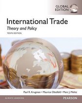
International Trade: Theory and Policy: Global Edition
This summary contains the complete content of the course International Trade and Investment. It covers chapters 1 to 12 of Krugman, Obstfeld and Melitz, Chapter 17 of Appleyard and field and the Lecture Slides used by the professor. I am a summary writer for Athena and passed this course with an 8....
Summary of the book 'International Trade: Theory and Policy' by Krugman, Obstfeld and Melitz
Full Summary International Trade and Investment
Summary of week 7 of International Trade and Investment
All for this textbook (8)
Written for
Universiteit van Amsterdam (UvA)
Economie
International Trade And Investment (6013B0465Y)
All documents for this subject (8)
2
reviews
By: taeyasmine • 2 year ago
By: borisbroekhuis • 3 year ago
Seller
Follow
larsadriaanse
Reviews received
Content preview
International Trade and Investment
Summary of Lectures and Slides
University of Amsterdam
Chapter 1: Introduction
An important insight in international economics is that there are gains from trade: when
countries sell goods to each other it is (almost) always to their mutual benefit, even when
some of them is more efficient at producing everything and when producers in the less-
efficient countries compete by paying lower wages. However, it is possible that international
trade may hurt particular groups within nations and hence affect the income distribution.
International trade analysis, which is studied in this course, focuses primarily on the real
transactions in the international economy: transactions involving tangible commitments of
economic resources.
Chapter 2: World Trade
There is a strong empirical relationship between the size of a country’s economy (GDP) and
the volume of both imports and exports. When looking at world trade as a whole,
economists have found that an equation of the following form predicts the volume of trade
between any two countries fairly accurately:
#
𝑇!" = 𝐴 ∗ 𝑌! ∗ $ !
"!
A = constant 𝑌! = country i’s GDP
T = value of trade between country i and j 𝑌" = country j’s GDP
D = distance between two countries
The above equation is known as a gravity model of world trade, and states that the value of
trade between any two countries is (ceteris paribus) proportional to the product of the two
countries’ GDPs and diminishes with the distance between the two countries. One of the
main applications of the gravity model is that it helps to identify anomalies in trade.
All gravity models estimated by economists show a strong negative effect of distance on
international trade. This partly reflects increased costs of transporting goods and services to
countries that are further away. Also, economists use the gravity model to assess the impact
of trade agreements on actual international trade: if an agreement is effective it should lead
to significantly more trading among its partners than would otherwise be predicted using
the standard gravity model.
Clearly, advances in technology (internet, airlines, etc.) have made it easier to trade
internationally (although gravity models still show a clear negative relation between
distance and trade). However, history shows that political forces can outweigh the effects of
technology. The world trade dropped between 1840-1914 due to political measures but
increased again for much of the 20th century. In that sense, a global economy we know today
is not new, and there have been two great waves of globalization (the first relying on the
railroads and telegraph). Since the mid-20th century tough, world trade as a share of
production has risen to unprecedented levels.
1
,Chapter 3: The Ricardian Model
Countries engage in trade because:
• They are different and hence can benefit from producing goods they are relatively
good at, and:
• To achieve economies of scale in production
This chapter focusses on the introduction of the concept of comparative advantage.
The reason that international trade produces an increase in world output is that it allows
each country to specialize in producing the good(s) in which it has a comparative advantage.
A country has a comparative advantage in producing a good if the opportunity cost of
producing that good in terms of other goods is lower in that country than it is in other
countries. Trade between two nations can benefit both if each country exports that good in
which it has a comparative advantage.
• The Ricardian Model
Suppose we are dealing with an economy (called Home) that has only one factor of
production (labor) and two goods: wine and cheese. The technology of Home’s economy can
be summarized by labor productivity in each industry, expressed as the unit labor
requirement: the amount of labor hours required to produce one unit. Note: the unit labor
%
requirement is the inverse of productivity (=&'!( *+,-. ./0&!./1/'(). The more a worker can
produce in an hour, the lower the unit labor requirement. We denote:
𝑎23 = 𝑢𝑛𝑖𝑡 𝑙𝑎𝑏𝑜𝑟 𝑟𝑒𝑞𝑢𝑖𝑟𝑒𝑚𝑒𝑛𝑡 𝑜𝑓 𝑤𝑖𝑛𝑒 𝑝𝑟𝑜𝑑𝑢𝑐𝑡𝑖𝑜𝑛
𝑎24 = 𝑢𝑛𝑖𝑡 𝑙𝑎𝑏𝑜𝑟 𝑟𝑒𝑞𝑢𝑖𝑟𝑒𝑚𝑒𝑛𝑡 𝑜𝑓 𝑐ℎ𝑒𝑒𝑠𝑒 𝑝𝑟𝑜𝑑𝑢𝑐𝑡𝑖𝑜𝑛
Because the economy in question has limited resources
(labor), we can graph the trade-off between the production of
the two goods by the following production possibility frontier->
If the economy would for example devote all its labor to wine
2
production, then it would produce + units of wine. In fact
#$
the economy can produce any combination that lies on the
PPF.
When the PPF is a straight line, the opportunity cost of cheese
in terms of wine is constant, and it is equal to the absolute
+
value of the slope: ;− + #% ;. Because producing another pound
#$
of cheese would require 𝑎24 labor hours and each of them could have alternatively be used
% +
to produced + units of wine, the opportunity cost of cheese in terms of wine is + #% .
#$ #$
To determine what Home will produce, we must look at relative prices of the two goods. Let
us first consider the situation where there is no international trade (autarky). As we assume
our economy is competitive, the supply of cheese and wine will be determined by the
movement of labor to whichever sector pays the highest wage. Therefore, we must equate
the marginal benefits (MB) of hiring a worker to the marginal cost (MC):
% %
𝑃5 ∗ + = 𝑤 and 𝑃6 ∗ + = 𝑤
#% #&
è The hourly wage equals the value of what a worker can produce in an hour.
2
,If:
7' +
7&
> + #% -> cheese wages are higher -> Home specializes in cheese production
#$
7' +#%
7&
<+ -> wine wages are higher -> Home specializes in wine production.
#$
7' +#%
7&
=+ -> both goods will be produced. In absence of trade, we must have this
#$
equality as home would have to produce both goods for itself. Under autarky, the relative
prices of the goods equal their relative unit labor requirements (opportunity cost).
Suppose now that there are two countries: Home and Foreign.
+ +∗
For now, the arbitrary assumption is made that + #% < +∗#%
#$ #$
meaning Home’s relative productivity in cheese is higher ->
Home has a comparative advantage in cheese. (Note: in this
example in the book Home is assumed to have an absolute
∗
advantage too as 𝑎24 < 𝑎24 . However, we need comparative
advantages to determine the pattern of trade). A PPF can be
drawn for Foreign too, this time with a steeper slope ->
When determining the relative price of cheese and wine after
trade, it is useful to keep track of relative supply and relative
demand. The next figure shows the world supply/demand curves for cheese relative to wine:
• The RS-curve:
7' +
If 7&
< + #% , there would be no supply of cheese as
#$
the relative price > opportunity costs. However, if
7' +
7
= + #% , the workers in Home are indifferent
& #$
between working in the cheese or wine industry,
meaning Home is willing to supply any relative
amount of the two goods. This can be seen at point
2. Remark that at this point, foreign would only
7 + ∗
produce wine as 7' > + #% ∗
& #$
+#% 7' + ∗
If, alternatively, + > 7 > + #% ∗ Home would
#$ & #$
specialize in cheese and Foreign in wine. Next, at
7' + ∗
7
= + #% ∗ we have another flat section as here
& #$
7'
Foreign is indifferent between producing cheese and wine. Finally, at a relative price >
7&
+#% ∗
+#$ ∗
both countries will specialize in cheese such that the relative supply of cheese will
become infinite.
• The RD-curve:
As the relative price of cheese rises, consumers substitute it for wine -> downward sloped
curve. Note that in equilibrium: RS = RD. Also, that the RD’-curve reflects a world that has a
larger preference for wine relative to cheese compared to the RD-curve.
3
, If we leave aside the possibility that one of the two countries do not completely specialize,
the normal result of free trade is that the relative price of the traded good (cheese) ends up
between the relative prices that would prevail under autarky. International trade hence leads
to the convergence of relative prices, resulting in each country specializing in the good in
which it has a comparative advantage.
International specialization and trade result in gains of trade. First of all, in our example
producing cheese and then trading it for wine (indirect production) is more efficient for
%
Home than producing wine directly. Home could namely produce + gallons of wine in an
#$
% 7
hour itself or produce +#%
pounds of cheese instead and then trading it for wine at 7' . As
&
% 7 % 7 +
long as + ∗ 7' > + or equivalently 7 ' > + #% (the case of specialization) the latter
#% & #$ $ #$
method makes Home better off.
Another way to see the mutual gains form trade is to note that trade and specialization will
lead to an expansion of consumption possibilities:
Clearly, once trade is allowed the economy of Home can consume more wine than
under autarky and simultaneously Foreign can consume more cheese. Trade has
enlarged the range of choice. Welfare of the whole world increases as labor is
allocated more efficiently.
• Note on the relative wages:
In our example the domestic workers are assumed to be more productive overall, and
therefore the wage in the domestic country must be larger than in the foreign
country (remember: perfect competition). If we assume an equilibrium at point 1 (see
previous supply/demand figure), and we have:
% %
+#%
∗ 𝑃5 = 𝑤 and +#$
∗ 𝑃6 = 𝑤 ∗
+ % 7 + ∗ : 7
In the example in the textbook, + #% = 9 > 7' > + #% ∗ = ;. Suppose now that 7' = 1, then
#$ & #$ &
6
w=12 but 𝑤 ∗ = 4, and the relative wage = 6 ∗ = 3. As it turns out, the wage rate lies between
+#$ ∗ ; 6 +#% ∗
the ratios of the two countries’ productivities in the two industries ( +#$
= 9 > 6∗ > +#%
=
6
6). It is precisely because 6 ∗ ends up between the relative productivities that each country
ends up with a cost advantage in one good. Because of its lower wage rate, Foreign has a
4
The benefits of buying summaries with Stuvia:
Guaranteed quality through customer reviews
Stuvia customers have reviewed more than 700,000 summaries. This how you know that you are buying the best documents.
Quick and easy check-out
You can quickly pay through credit card or Stuvia-credit for the summaries. There is no membership needed.
Focus on what matters
Your fellow students write the study notes themselves, which is why the documents are always reliable and up-to-date. This ensures you quickly get to the core!
Frequently asked questions
What do I get when I buy this document?
You get a PDF, available immediately after your purchase. The purchased document is accessible anytime, anywhere and indefinitely through your profile.
Satisfaction guarantee: how does it work?
Our satisfaction guarantee ensures that you always find a study document that suits you well. You fill out a form, and our customer service team takes care of the rest.
Who am I buying these notes from?
Stuvia is a marketplace, so you are not buying this document from us, but from seller larsadriaanse. Stuvia facilitates payment to the seller.
Will I be stuck with a subscription?
No, you only buy these notes for $6.64. You're not tied to anything after your purchase.