Lecture 1.1 - t-test, confidence interval & sample size
Example:
We want to compare population means of two populations; the population of diabetic
patients following diet A and diet B. The diabetic patients are the units.
We cannot look at all patients, but make a guess about the difference by looking at two
random samples from the populations the two samples follow from one random sample
of patients and randomisation over the two treatments.
Experimental study = experiment where treatments can be randomly assigned to
experimental units.
We want to compare the population means μ1 and μ2.
The research hypothesis is that μ1 and μ2 are different; this will be the alternative
hypothesis, so H a : μ1−μ2 ≠ 0. The null hypothesis will be H 0 : μ1−μ2=0.
σ2 = variance = measures the average degree to which number is different from the mean.
The test statistic measures how well the data match up with H0.
ŷ (sample mean) = estimator for μ (population mean)
s (sample standard deviation) = estimator for σ (standard deviation)
s2 (pooled variance estimate) = estimator for σ2 (variance) the variance of several different
populations with different means for the populations.
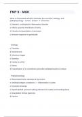
Very positive t
suggests μ1−μ 2>0 , so
reject H0.
Very negative t
suggests μ1−μ 2<0 , so
reject H0 too.
But when it’s negative/positive enough? Rejection Region = the outcomes of t that lead
to rejection of H0.
Degrees of freedom (df) = represent how many values involved in a calculation have the
freedom to vary.
df = (n1- 1) + (n2 – 1)
To determine the rejection region we need to know the distribution of t under H 0, to decide
which values of t are rare.
1
,LET OP! A t- distribution is more flat than a normal distribution.
If the question concerns the entire population as it is distributed normal distribution
should be used.
If question concerns the mean of the population the t-statistic may be used
P-value = the probability under H0 for the outcome of test statistic t and anything more
extreme (supporting Ha). LET OP! Two sided p-value? 2x the p-value found.
P-value ≤ α reject H0, Ha has been shown
P-value > α do not reject H0
estimator−value of parameter under H 0
t=
SE
The estimate is the difference between two sample means
Value from H0 is often zero
Standard error is standard deviation of the estimator
One sample t-test
1 random sample, 1 variable interest in single population mean μ
Example: sample from population of Dutch people
y = daily salt consumption of a person
μ = population mean for daily salt consumption of Dutch people
ŷ−6
t= 2
H0: μ = 6, Ha: μ > 6, s
√
n
Paired t-test
1 random sample, 2 variables interest in difference between population means μ1−μ 2
Example: sample of patients with blood pressure disorder
y = blood pressure, measured before and after medication
μ1/2 = population means before and after medication
d−0
t= 2
d = x – y, H0: μd = 0, Ha: μd > 0, s
√
n
Confidence Interval = set of values for which the null hypothesis is accepted alle
waarschijnlijke waarden voor μ1−μ 2
2
,CI =estimator ± t α (constant ) × SE
2
LET OP! Rejection Region is expressed in t. CI is expressed in the variable you need to know.
Door de α te veranderen, verander je de betrouwbaarheid van het interval. LET OP! Bij een
kleinere confidence interval heb je een hogere betrouwbaarheid nodig verhoging van de
sample size waardoor de SE kleiner wordt; hoe smaller het interval, hoe nauwkeuriger!
In a (very) large experiment, a difference could be significant, while a narrow interval, and a
small estimate, may tell you that the difference is of no practical importance. Statistically
significant and practically significant is not always the same!
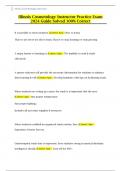
At a given α, for smaller β a
larger sample size n is required.
Power calculation = the probability of correctly rejecting the null hypothesis when it is false
Calculate how big your sample size needs to be:
1) Based on tests; zo veel power nodig voor een significant verschil
Use a two-independent sample t-test
Either be negative or positive two sided alternative hypothesis
Equation six:
Suppose probability of 0.95, β = 1 – 0.95
= 0.05
n = 65? We need at least 65 patients for each
diet, so 130 patients in total.
2) Estimate the difference
We want a small width of a confidence interval error margin (E) = half of
the width of the interval.
When the true value is in the interval, the true value and the estimate will
differ less than E.
Interested in a confidence interval
Interval responds to a two-independent samples t-test
Equation nine:
N = 77? We need at least 77 patients for each
diet, so 154 in total.
LET OP! Afronden naar boven; 76.4 wordt 77.
3
, Lecture 1.2 – Analysis of proportions and tables
Example – one proportion & one sample
The proportion of binge drinking among students is 0.44. Let π be the proportion of students
that engage in binge drinking at a particular university. Is π larger than 0.44?
Experimental units = students
Response = student is a binge drinker or not (LET OP! Amount doesn’t matter)
Basic observations are binary 1 if student is a binge drinker and 0 if not.
Population mean of binary data is also a population proportion, here the proportion of binge
drinkers in the student population. This is also the probability that a randomly selected
student is a binge drinker for that reason we use symbol π.
DUS: Gemiddelde van 0’tjes en 1’tjes is in feite ook de proportie.
TEST STATISTIC
H 0 :π =0.44 H a :π >0.44
This is a one-sided alternative hypothesis. The test statistic is number of observed binge
drinkers Y. When Y is too large, we reject H0.
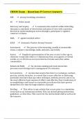
Suppose Y = 240
P−value=P ( y ≥240 ) for π = 0.44
P-value = is de kans dat je testresultaten vindt dat H0 waar is, of extremer.
¿ aantal successen( y )
π= estimate for π
aantal deelnemers(n)
Calculate 0.95-confidence
interval:
4
Example:
We want to compare population means of two populations; the population of diabetic
patients following diet A and diet B. The diabetic patients are the units.
We cannot look at all patients, but make a guess about the difference by looking at two
random samples from the populations the two samples follow from one random sample
of patients and randomisation over the two treatments.
Experimental study = experiment where treatments can be randomly assigned to
experimental units.
We want to compare the population means μ1 and μ2.
The research hypothesis is that μ1 and μ2 are different; this will be the alternative
hypothesis, so H a : μ1−μ2 ≠ 0. The null hypothesis will be H 0 : μ1−μ2=0.
σ2 = variance = measures the average degree to which number is different from the mean.
The test statistic measures how well the data match up with H0.
ŷ (sample mean) = estimator for μ (population mean)
s (sample standard deviation) = estimator for σ (standard deviation)
s2 (pooled variance estimate) = estimator for σ2 (variance) the variance of several different
populations with different means for the populations.
Very positive t
suggests μ1−μ 2>0 , so
reject H0.
Very negative t
suggests μ1−μ 2<0 , so
reject H0 too.
But when it’s negative/positive enough? Rejection Region = the outcomes of t that lead
to rejection of H0.
Degrees of freedom (df) = represent how many values involved in a calculation have the
freedom to vary.
df = (n1- 1) + (n2 – 1)
To determine the rejection region we need to know the distribution of t under H 0, to decide
which values of t are rare.
1
,LET OP! A t- distribution is more flat than a normal distribution.
If the question concerns the entire population as it is distributed normal distribution
should be used.
If question concerns the mean of the population the t-statistic may be used
P-value = the probability under H0 for the outcome of test statistic t and anything more
extreme (supporting Ha). LET OP! Two sided p-value? 2x the p-value found.
P-value ≤ α reject H0, Ha has been shown
P-value > α do not reject H0
estimator−value of parameter under H 0
t=
SE
The estimate is the difference between two sample means
Value from H0 is often zero
Standard error is standard deviation of the estimator
One sample t-test
1 random sample, 1 variable interest in single population mean μ
Example: sample from population of Dutch people
y = daily salt consumption of a person
μ = population mean for daily salt consumption of Dutch people
ŷ−6
t= 2
H0: μ = 6, Ha: μ > 6, s
√
n
Paired t-test
1 random sample, 2 variables interest in difference between population means μ1−μ 2
Example: sample of patients with blood pressure disorder
y = blood pressure, measured before and after medication
μ1/2 = population means before and after medication
d−0
t= 2
d = x – y, H0: μd = 0, Ha: μd > 0, s
√
n
Confidence Interval = set of values for which the null hypothesis is accepted alle
waarschijnlijke waarden voor μ1−μ 2
2
,CI =estimator ± t α (constant ) × SE
2
LET OP! Rejection Region is expressed in t. CI is expressed in the variable you need to know.
Door de α te veranderen, verander je de betrouwbaarheid van het interval. LET OP! Bij een
kleinere confidence interval heb je een hogere betrouwbaarheid nodig verhoging van de
sample size waardoor de SE kleiner wordt; hoe smaller het interval, hoe nauwkeuriger!
In a (very) large experiment, a difference could be significant, while a narrow interval, and a
small estimate, may tell you that the difference is of no practical importance. Statistically
significant and practically significant is not always the same!
At a given α, for smaller β a
larger sample size n is required.
Power calculation = the probability of correctly rejecting the null hypothesis when it is false
Calculate how big your sample size needs to be:
1) Based on tests; zo veel power nodig voor een significant verschil
Use a two-independent sample t-test
Either be negative or positive two sided alternative hypothesis
Equation six:
Suppose probability of 0.95, β = 1 – 0.95
= 0.05
n = 65? We need at least 65 patients for each
diet, so 130 patients in total.
2) Estimate the difference
We want a small width of a confidence interval error margin (E) = half of
the width of the interval.
When the true value is in the interval, the true value and the estimate will
differ less than E.
Interested in a confidence interval
Interval responds to a two-independent samples t-test
Equation nine:
N = 77? We need at least 77 patients for each
diet, so 154 in total.
LET OP! Afronden naar boven; 76.4 wordt 77.
3
, Lecture 1.2 – Analysis of proportions and tables
Example – one proportion & one sample
The proportion of binge drinking among students is 0.44. Let π be the proportion of students
that engage in binge drinking at a particular university. Is π larger than 0.44?
Experimental units = students
Response = student is a binge drinker or not (LET OP! Amount doesn’t matter)
Basic observations are binary 1 if student is a binge drinker and 0 if not.
Population mean of binary data is also a population proportion, here the proportion of binge
drinkers in the student population. This is also the probability that a randomly selected
student is a binge drinker for that reason we use symbol π.
DUS: Gemiddelde van 0’tjes en 1’tjes is in feite ook de proportie.
TEST STATISTIC
H 0 :π =0.44 H a :π >0.44
This is a one-sided alternative hypothesis. The test statistic is number of observed binge
drinkers Y. When Y is too large, we reject H0.
Suppose Y = 240
P−value=P ( y ≥240 ) for π = 0.44
P-value = is de kans dat je testresultaten vindt dat H0 waar is, of extremer.
¿ aantal successen( y )
π= estimate for π
aantal deelnemers(n)
Calculate 0.95-confidence
interval:
4