Summer MGT 6203 MID EXAM
PART2 – CODING
Week 1
Use the inbuilt dataset ‘longley’ for questions 1 and 2.
Q1) Fit a linear regression model with ‘Employed’ as the response
variable and all other variables (except ‘Year’) as predictors. What are the
significant predictors at 10% significance level?
A. GNP
B. GNP, Armed.Forces
C. GNP, Unemployed, Population
D. None of the predictors are significant at 10% significance level
Solution:
model1 = lm(Employed~.-Year, data = longley)
summary(model1)
##
## Call:
## lm(formula = Employed ~ . - Year, data = longley)
##
## Residuals:
## Min 1Q Median 3Q Max
## -0.55324 -0.36478 0.06106 0.20550 0.93359
##
## Coefficients:
## Estimate Std. Error t value Pr(>|t|)
## (Intercept) 92.461308 35.169248 2.629 0.0252 *
## GNP.deflator -0.048463 0.132248 -0.366 0.7217
## GNP 0.072004 0.031734 2.269 0.0467 *
## Unemployed -0.004039 0.004385 -0.921 0.3788
## Armed.Forces -0.005605 0.002838 -1.975 0.0765 .
## Population -0.403509 0.330264 -1.222 0.2498
## ---
## Signif. codes: 0 '***' 0.001 '**' 0.01 '*' 0.05 '.' 0.1 ' ' 1
##
## Residual standard error: 0.4832 on 10 degrees of freedom
## Multiple R-squared: 0.9874, Adjusted R-squared: 0.9811
## F-statistic: 156.4 on 5 and 10 DF, p-value: 3.699e-09
From the p-value, we can see that GNP and Armed.Forces are significant at 10%
significance level.
Q2) What can you say about multicollinearity in this model?
a. The model does not exhibit multicollinearity
b. The model exhibits multicollinearity due to high correlation between GNP,
Armed.Forces
, c. The model exhibits multicollinearity due to high correlation between GNP,
GNP.deflator and population
d. The model exhibits multicollinearity due to high correlation between GNP.deflator,
Unemployed
Solution:
vif(model1)
## GNP.deflator GNP Unemployed Armed.Forces Population
## 130.829201 639.049777 10.786858 2.505775 339.011693
Yes, looking at the VIF table, we can see that GNP, GNP deflator and population have high
VIF values indicating multicollinearity issue. We may also look at the correlation matrix
to come to the same conclusion.
cor(longley[,-6])
## GNP.deflator GNP Unemployed Armed.Forces
Population
## GNP.deflator 1.0000000 0.9915892 0.6206334 0.4647442
0.9791634
## GNP 0.9915892 1.0000000 0.6042609 0.4464368
0.9910901
## Unemployed 0.6206334 0.6042609 1.0000000 -0.1774206
0.6865515
## Armed.Forces 0.4647442 0.4464368 -0.1774206 1.0000000
0.3644163
## Population 0.9791634 0.9910901 0.6865515 0.3644163
1.0000000
## Employed 0.9708985 0.9835516 0.5024981 0.4573074
0.9603906
## Employed
## GNP.deflator 0.9708985
## GNP 0.9835516
## Unemployed 0.5024981
## Armed.Forces 0.4573074
## Population 0.9603906
## Employed 1.0000000
We can see that GNP, GNP deflator and population are highly correlated causing
multicollinearity issue.
Week 2
Q3) The trees dataset contains the girth (diameter), height, and volume for black cherry trees.
Download the dataset in R using the command “data(trees)”. Create two Linear-Linear
models. The first model should use girth to predict volume, and the second model should use
height to predict volume. What is the Adjusted R-Squared for each model.
A. 0.9471, 0.4334
B. 0.8243, 0.3265
C. 0.9331, 0.3358
D. 0.9798, 0.3292
,
PART2 – CODING
Week 1
Use the inbuilt dataset ‘longley’ for questions 1 and 2.
Q1) Fit a linear regression model with ‘Employed’ as the response
variable and all other variables (except ‘Year’) as predictors. What are the
significant predictors at 10% significance level?
A. GNP
B. GNP, Armed.Forces
C. GNP, Unemployed, Population
D. None of the predictors are significant at 10% significance level
Solution:
model1 = lm(Employed~.-Year, data = longley)
summary(model1)
##
## Call:
## lm(formula = Employed ~ . - Year, data = longley)
##
## Residuals:
## Min 1Q Median 3Q Max
## -0.55324 -0.36478 0.06106 0.20550 0.93359
##
## Coefficients:
## Estimate Std. Error t value Pr(>|t|)
## (Intercept) 92.461308 35.169248 2.629 0.0252 *
## GNP.deflator -0.048463 0.132248 -0.366 0.7217
## GNP 0.072004 0.031734 2.269 0.0467 *
## Unemployed -0.004039 0.004385 -0.921 0.3788
## Armed.Forces -0.005605 0.002838 -1.975 0.0765 .
## Population -0.403509 0.330264 -1.222 0.2498
## ---
## Signif. codes: 0 '***' 0.001 '**' 0.01 '*' 0.05 '.' 0.1 ' ' 1
##
## Residual standard error: 0.4832 on 10 degrees of freedom
## Multiple R-squared: 0.9874, Adjusted R-squared: 0.9811
## F-statistic: 156.4 on 5 and 10 DF, p-value: 3.699e-09
From the p-value, we can see that GNP and Armed.Forces are significant at 10%
significance level.
Q2) What can you say about multicollinearity in this model?
a. The model does not exhibit multicollinearity
b. The model exhibits multicollinearity due to high correlation between GNP,
Armed.Forces
, c. The model exhibits multicollinearity due to high correlation between GNP,
GNP.deflator and population
d. The model exhibits multicollinearity due to high correlation between GNP.deflator,
Unemployed
Solution:
vif(model1)
## GNP.deflator GNP Unemployed Armed.Forces Population
## 130.829201 639.049777 10.786858 2.505775 339.011693
Yes, looking at the VIF table, we can see that GNP, GNP deflator and population have high
VIF values indicating multicollinearity issue. We may also look at the correlation matrix
to come to the same conclusion.
cor(longley[,-6])
## GNP.deflator GNP Unemployed Armed.Forces
Population
## GNP.deflator 1.0000000 0.9915892 0.6206334 0.4647442
0.9791634
## GNP 0.9915892 1.0000000 0.6042609 0.4464368
0.9910901
## Unemployed 0.6206334 0.6042609 1.0000000 -0.1774206
0.6865515
## Armed.Forces 0.4647442 0.4464368 -0.1774206 1.0000000
0.3644163
## Population 0.9791634 0.9910901 0.6865515 0.3644163
1.0000000
## Employed 0.9708985 0.9835516 0.5024981 0.4573074
0.9603906
## Employed
## GNP.deflator 0.9708985
## GNP 0.9835516
## Unemployed 0.5024981
## Armed.Forces 0.4573074
## Population 0.9603906
## Employed 1.0000000
We can see that GNP, GNP deflator and population are highly correlated causing
multicollinearity issue.
Week 2
Q3) The trees dataset contains the girth (diameter), height, and volume for black cherry trees.
Download the dataset in R using the command “data(trees)”. Create two Linear-Linear
models. The first model should use girth to predict volume, and the second model should use
height to predict volume. What is the Adjusted R-Squared for each model.
A. 0.9471, 0.4334
B. 0.8243, 0.3265
C. 0.9331, 0.3358
D. 0.9798, 0.3292
,