finding the average/ mean of sets -
add all the values $ divide by the amount of no .
U added
averages :
① { 2 7 3 5 }
avg / mean of , , ,
,
a
◦
: 17/5 = 3 . 4
② R 54
avg price of R42
,
R 50
,
◦
: 421-501-54 = R 48 67
,
3
continuous function
^
y areas of roam -
wax
↳ under the
ya area of rectangle = area curve
, under
area curve
ya c
=
✗
'
under curve
avg Val =
area
C
b
c
avg Val = ¥a f a
fix) doc
example
① Average value
7
of fact = od over [ 3,7]
§ = ÷ JOE
3
doc
area under
¥?:::
=
Ya [ x% ]} curve =
=
'
it [% -
3% ] rectangle in
.
=
79/3 = 26 ,
3
S
,2.) savings account , 3% interest compounded continually
At year end bonus = 1% of average balance in account during the year -
Deposit R10 000 at start, what is bonus at end of year 1?
" °"
s cont .
comp .
A- (f) =
10000 @
b
avg balance =
A- =¥a
'
J Alt) dt
a
= ¥0 J 10000 @
" ° "
dt
0
[ t.org ];
◦ ' 03£
=
10000 @
10151,51
=
Bonus = It × 10151,51
=
R 101,52
, moving averages (discrete & continuous)
when we have a sequence of data points Iz Iz the values are likely to
,
JC ,
, ,
-
. . ✗ 20
jump up and down. This makes it difficult to discern if there is a trend
•
: we use moving averages to:
- smooth it irregularities
- show trends
NB! the higher the n the smoother the plot but the greater the lag
EXAMPLE:
1.) find the 5 day moving average
SO! to move the average we construct a new sequence of data by taking the
average of the first 5 points
:⊖
÷/É::::
Moving
22.2 22.8 23.4 24.4 23,6 23,6
20
i. e. f- (5) =É[¥ ,
Xi then f- (6) =É%=z0Ci . . .
f- ( 201=5 [ i. *
Oci
: the n-unit moving average of a function:
✗ → endpoint
fix tnffcxldx-
_
↓ 2C n-
n
OE
an → begin point
ifeng.tn
, "
avg on
[a. b)
Gee subint points
ya
f. f ca
=
+ Éox )
f⇐ ,
f- ≈
(ft tfz
600C
t - - -
f- 6
] ox
a
'
b ¥
t.floxtfzoxt.r.tt# n
b- a
§ ≈ [
in
fi ox
↳ reimann sum !!
b- a
¥4 fi
9
As
§ S fix> dx
° "
n →
a .
=
¥ . =
↳
b- a
b- a
Example :
f
3
① C) ✗ x2 30C 3 unit
moving
+
avg
= -
,
x
§ =
↳
f ( Est E
'
-
3-c) It
x -3
"
43 [ Yat ↳ % ]
" '
=
+ t 3- t
x 3
-
= (K2 I
"
t Ya 2C
} _
tz x2 ) -
( Hz ( x 3) -
"
t Yq (x 3)-
3
hex-312 )
'
-
Ya (
f-
}
↳c) =
ax _
14 x2 + 122C +
3)
↳
Nt "
,continuous income streams
"
FU =P Vert
compounding !!
→
RK)
↳ revenue
rand
.
per day ,
t in
days
———-formula ————————————————
O
total revenue
b
total rev = TV = f Rtt ) dt
↳
a
total income over [ a. b ]
•
future value (incl interest)
'
future value = FV = fa
R (E) er
#"
dt
0
present value
"
[
↑
Puerto $
a) "
Rctjrlb
- -
FU =
↳
in
yrs
FU =
dt
a
f
"" ' "" '
-
:
Pver =
Rlt) er dt
a
b
f R (f) er
1
" " -
PU =
de e-
' b- a)
.
a
[
re rb + ra
R (f) erb
- -
=
dt
:
f R / Her
""
dt
=
a
present value = PV = ! a
R (E) er
"
de
,EXAMPLE: total value
1.) sales income from 1 nov to 31 jan, 92 days given by
R(t)= 30000 + 45t - 0,5t rand per year
total income over period?
time interval [0,92]
n - sub intervals [ tic - i
,
tic ] of length Ot
•
: revenue in any sub interval [ tic - i
,
tic ] is approx
R (tic ) -
i
Ot
Add or all sub intervals
total income = Rlto ) Ott R ( Ei ) Ott
- - .
+ R ( En - 1) Ot
92 ↳ left reiman sum
let n → a total income =
frltldt
0
92
[
=
(30001-451--0.5-4) dt
R 336659
=
EXAMPLE: future value
2.) Future value continuous income stream, deposited into account paying interest
(continuous compounding)
- ↳ Fu =P Vert
interest 5% pa, balance at end of jan?
2
$ R (t) = 3000 + 45-6 -
0,5 C-
S [0 , ]
92
,
sub int [ tic -
ist ] ,
Ot
; rev ≈ Rltk 1) -
Ot
deposited ( PV )
R
◦ ◦ s ( 92 -
tic -11/365
ACK 1)
'
-
=
of @
add for all the sub intervals
, Int earned 92 tk , days
-
:
92ggᵗg Years
↳ R (-1--0) Of @
0105 ( 92 1365 t
R( of e.
" ◦
sC92- 136% .
. .
" ◦ scaz -⇐ / 365
+ R ( € of e
92
f
5 '" "
1365dg
◦ ' ◦ -
As n → 0
,
balance Rft) @
0
EXAMPLE: present value
3.) Inga was injured and can no longer work. As a result she is awarded the present
value of income that she would have receive over the next 20 yrs. Her income at the
time of injury was $100000 /yr increasing by $5000 / yr. What will the amt she is
awarded be assuming continuous income and a 5% interest rate.
PU= [ Rfllerla -
"
dt
tin
↳
years
20
- IBP :
§( )e%◦( Hdt °
So PU f-
-
1000001-5000-1
g'
"°"
=
20T£ e-
=
=
'
◦
g. I
= ""
1. e-
5000%20 g.
=
"" "
E) e- dt
=
+ -
aos
"
5000¢20 f) °ˢᵗ
'°ˢᵗ
f
°
e-
"
1. C-
+
-
=
-
0,0s -
0,05
=
$1,792,723,35
,Improper integrals
improper integral if function is undefined in given range
definite :
↑ a
fix doc
indefinite :
f fix ) doc
0
if
" "
finite =
converges
uded/ infinite =
"
diverges
"
↳ no upper or lower limit
◦
aka no boundaries .
what if:
1.) a or b not finite
[ fix ] da := i
M→x
§ fix) dx
this allows us to evaluate the integral and then take the limit → ☒
b
I.Jfcxldx :=
ei
m→ .
. f. fixate
fix )dx : =
§ .
fcxsdx + § .
fcx) dx
= for a conveniently chosen c, provided that both integrals on RHS converge
2.) F(x) not continuous on [a, b]
↳
§
-
2
2
↳
doc
✗ not defined @ 0
integral diverges when your answer is: ✗ or -
✗
integral converges when your answer is: normal
, type 1: from a definite to an indefinite. Approaches 0
;
-
x
type 2: definite range but integrals not defined
Example :
type I Infinite limits of integration .
j ¥2
•
,
dx =
li
M→ 0
JIE ,
da
= li
→ •
1- ÷ ] ?
=
e.
m → a
⇐ -
t :-|]
=
% .
C- In + I ] .
=
I
0
similarly :
§ - A
e-
"
doe =
him →
_ •
/
M
e-
"
dx
=
I'm →
•
[ e-
"
I
=
I C- I + e-
m
)
M → -
A
=/
e- 1-01=0
= -
I t ✗
=
@
limit
'
.
'
does not exist $ integral diverges .
, It definite / improper integrals
Example :
type inter grab
integrands that become infinite
§ II doc j
•
on lo ,
i
] ¥ is defined
-
0
•
as ✗ → 0 → a
,
[# doc : lie⇐
door→ Ot
[ r
= tr
↳ ◦
+
[ 2K ]!
=
↳ + ( 2 -
2 F)
§ Éidx =
. .
_
§¥ ,
doc
=
[
2
Ézdx +
% ¥2 doc
r
=
[
2
¥ dx =
li
'
f 'xadx = I
r→◦
.
Ex ]: =
f- ÷ -
C- ÷ )]
r→ 0
,
=
liftr→o
-
-
E)
= 0 -
£ =
a
÷ limit does not exist
÷
[
-2
Édx diverges
→
if one
then
part
the
diverges
whole
thing diverges
NB ! !
3
f. ¥2
'
doc ≠ f- ¥] z
= -
§
→
¥ is
always tire . : area under
graph ≠ 've