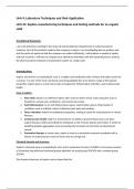
Pr[outcome1] / Pr[evidence] The smaller the value of k, the more likely the model to overfit.
Pearson ∈ [-1, 1] Pr[evidence] is constant. Calculate the green part for both outcomes first • Stratification procedure: ensures that decision class distrib. of a given
and then obtain Pr[evidence]. sample is proportionally similar to decision class distrib. of whole pop.
#!∘ #∘" % NB assumes that features have the same importance and are independent. • Random search: explores a set of possible combinations. It might overlook
"#!" $ % good models but is faster and usually gets the job done. Can be used to
Chi-sq. association χ! = ∑*+() ∑&'() #
#!∘ #∘"
Real-life yes Real-life no pinpoint a range of promising values for hyperparams, to then apply grid
#
-> H0 is false -> H0 is true search on a narrower range to find the best combination.
Steps in data pre-processing:
Bias: diffrence btwn the predictions made by the algorithm and the ground truth
• Imputing missing data: Predict yes True positive False positive Variance: difference in the predictions when fitting the model on data from the
o Remove the feature → limited number of features
-> Reject H0 Type I error same distr. (diff btwn train and validation accuracy)
o Remove the instance → limited number of instances
o Replace missing values → introduce noise P = 1−β P = α Error of commiss.
• Standardizing numerical features (feature scaling) Predict no False negative True negative
• Encoding categorical values -> Fail to reject H0 Type II error
o Label encoding: assign integer to category, for var.s with ordinal relations
P = β Error of omission P = 1−α
o One-hot e.: basically dummy var.s → increases problem dimensionality
• Analyzing outliers 𝑃𝑟𝑒𝑐𝑖𝑠𝑖𝑜𝑛 =
23
𝐴𝑐𝑐𝑢𝑟𝑎𝑐𝑦 =
23025
• Tackling class imbalance 23043 67689
o Undersampling: select some instances from majority class 23 3:;<=>=7?∗A;<899
o Oversampling: create new instances (copies) for the minority class 𝑅𝑒𝑐𝑎𝑙𝑙 = 𝐹1 = 2 ∗
23045 3:;<=>=7?0A;<899
o SMOTE: creates synthetic instances in the neighborhoods of instances
Use precision: if misclassification is costly, to avoid type I error
from minority class → might induce noise
e.g. wastage is pref. over sudden disaster (don’t convict the innocent)
Distance functions Use recall: if misidentification is costly, to avoid type II error
Euclidean e.g. punishing is preferred over overlooking (identify hijackers)
Manhattan Fβ-score:
Hamming dist s.t. Underfitting: model performs poorly on the training data; overfitting: model
performs well during training and possibly validation, but poorly during testing.
'!#$!"# ( '!#$!$%
Diversity in number of dimensions: 𝐷𝑖𝑣 = log ( )
'!#$!$%
Dimensionality reduction (advantages): better visualization, lower risk of
• Generalization capability (= out-of-sample evaluation): model’s perfor- overfitting, higher model efficiency (e.g. shorter training times).
mance on unseen data, provides evidence on usability of the model in practice
o Training set: used to build the model
• Filter methods:
o Validation set: used to determine the best hyperparameters
o require an information criterion (e.g., info.gain, correlation, chisq.
o Test set: used to assess the model’s generaliz. capab. for unseen data
(dependency), stat.signif.test) to rank features,
Random forest: uses bagging which performs random sampling with replacement from the o don't use ML models (i.e. model training) to decide whether a feature
original dataset. Furthermore, it makes random feature selection to grow trees (normally should be kept -> faster and computat.ly less expensive;
btwn 100 and 500). After aggregating the outputs, the most popular decision class in the
forest is assigned to the new instance. Suitable for prob.s with high variance in prediction. • Wrapper methods:
Boosting: assigns more relevance (large weights) to more difficult instances. Next, retrain o use ML models – computat.ly more expensive, (i.e., train-test procedure ->
the classifier with the new weights. Bagging is parallel, while boosting is sequential. define classifier -> determine performance score)
o Forward selection: starts with an empty set of features, iteratively chooses the best
Information gain Nested k-fold cv: feature (remaining) among the best features and adds it to the new set. Backward elim.:
starts with a full set and iteratively removes the worst feature remaining in the set.
(log2!) info(feature ← instance) = entropy(Pinst) o Recursive feat. elimination: iteratively develops models with the remaining
features after removing the least significant one(s). The process is repeated
𝑛! until the desired number of features is obtained.;
𝑖𝑛𝑓𝑜(𝑓𝑒𝑎𝑡𝑢𝑟𝑒) = . 𝑒𝑛𝑡𝑟𝑜𝑝𝑦(𝑃!"#$ )
𝑛 • Embedded methods:
𝑜𝑢𝑡𝑐𝑜𝑚𝑒% 𝑜𝑢𝑡𝑐𝑜𝑚𝑒& o have the advantage that the same model used for solving the ML problem
𝑖𝑛𝑓𝑜(𝑟𝑜𝑜𝑡) = 𝑒𝑛𝑡𝑟( ; ;…) also determines the most important features (e.g., a regression model or a decision tree)
∑ 𝑜𝑢𝑡𝑐𝑜𝑚𝑒 ∑ 𝑜𝑢𝑡𝑐𝑜𝑚𝑒
o mostly use regr. methods w regularization: add a penalty term to the
gain(feature) = info(root) – info(feature) error/loss function, pushing some feature coefficients to exactly zero;
e.g. info(outlook ← sunny) = entropy([2/5, 3/5]) • Feature extraction methods:
info(outlook ← overcast) = entropy([4/4, 0/4]) o extract features that do not carry any semantic information and might not be
easily interpretable in the context of the problem domain;
Naive Bayes o example, PCA: transforms the orig. variables into a set of new uncorrelated
for yes: 2/9 * (3/9)3 * 9/14 = 0.0053 variables = principal components. They are lin. combinations of the original
for no: 3/5 * 1/5 * 4/5 * 3/5 * 5/14 = 0.0206 ones and capture the max. amount of variance in the dataset. Princip.
,.,,./
= > Pr[𝑦𝑒𝑠|𝐸] = Comps are weighted by relevance.
,.,,./0,.,!,1

