Econometric Methods with Applications in Business and Economics
This comprehensive handwritten summary of Econometrics Methods with Applications covers key topics and concepts, derived from both lectures and the textbook. The notes include detailed explanations on linear regression models, least squares estimation, multivariate regression analysis, and the clas...
Test Bank for Introductory Econometrics A Modern Approach, 5th Edition by Jeffrey M. Wooldridge
All for this textbook (10)
Written for
Universiteit van Amsterdam (UvA)
Econometrics & Data Science
6012B0374Y
All documents for this subject (1)
Seller
Follow
lucia2001
Content preview
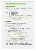
Week 1: linear regression with one regressor
7 1
.
Linear Regression model
we want to find a line that best fits the given data ,
consider the
linear model in parameters :
li =
2
+ BKki + Ei ,
=
1 ...
where : Yi : dependent variable
Chi :
explanatory variable
n :
sample size
Ei :
error term that captures the variation in yi not explained by
usually, Coefficient Bi can be interpreted as partial marginal effect
Bi =
0ESYilChi . . . . . Thkin] K = 1
,
. .
.,
K
8 k,
1 2
. .
Least Squares
the most simple linear model I
has explanatory variable :
Hi = x +
BXli + Ei i = 1,
...,
N
where we want to find < B use OLS -
· minimise the sum of squared residuals
the residual :ei Yi-x-Bli =
12 . B) =
argmin & 2Sn(x . B) =
argmin E (Yi-x .
Bi e
now ,
take partial derivatives to
get B :
8 (Sn(d B) ,
= -
2 [F .
(Yi X-Bl(i)
- =
O
8
.. 2
1((yi B[((i) y B
=
=
- -
0 (Sn(X B) 2 [i (Yi x-Bli) Ki O
-
=
= -
,
OB
*
plug in value for : [ .. <(i)(yi-y) -B((i ii) - =
0
:
B =
[i < i(yi -Y) =
[iKli -
< i) (yi i) -
[i xi(ki TL) [i ((i 5)
:
- -
variables transformed *= Y C
·
When are s t .
.:
Yi dy +
by Yi & = + balLi
B
=by
↑
&** =
*
then axB byi
dy-by
+
adding constants to yidcli doesn't influence but multiplying all Yid K:
scales B (up/down) ,
while I absorbs all location changes in <id yi
, .
1 3 .
Binary regressor
When xi =
Di is a
dummy binary e .
g. male or female ,
then :
assuming n =
no +
n, where n =
[Di (#obs where Di . = 1)
* [: Mei M135 - MoJo Yo
-
=
Di(yi-y) = -
My = (n -
=
J .
-
[i Di (Di-D) n
-
,
n B n
-
M
I
j B5 y Yo) 5 Mej Mojo 14 40 To
15
(M)
+
-
-
-
= =
-
= - =
,
1 .
4 Goodness of fit R2
> fitted value
generic decomposition of data :
Yi =
Yi + : > residuals
SST =
SSE + SSR
* fitted value i : = < +
B : (the projected value of Yi on the line < + B <li
* residual ii : =
yi-x-Bxi (what remains once we've done the projection)
Liyie 0 =
they are orthogonal to each other (irrespective of the regressor)
* the OLS estimator minimises the SSR4 maximises the SSE
the ratio of explaineda unexplained variance of yi is :
SST = SSE + SSR
SST SST 58 T
explained variance :
SSE =
R2 maximised want to :·
explain yi as best
SST as we can with
2i
unexplained variance : SSR = 1-R2
SST
· When multiple models choose one with highest R2
comparing ,
=>
high R2 doesn't guarantee better predictions doesn't say anything about out-of- :
sample predictions to choose a
good model ,
must consider :
4) in- sample
(2) Out-of-sample
1 5 .
Linear model motivation (3) non-statistical considerations
1. Reduced form models are driven by heuristic observations about potential relationships
between certain variables. These models are hard to make predictions outside of the obs.
at hand. They focus on internal validity.
2. Structural form models are generally derived from certain types of economic models (e.g.
profit maximisation). They are restrictive but can tell us a lot about out of sample
prediction. They focus on external validity.
3. Microeconomics focusses on individual consumers, firms & micro-level decision makers etc.
It uses disaggregated cross-section & panel data.
4. Macroeconomics focusses on price levels, money supply, exchange rates, output,
investment, economic growth etc. It uses aggregated time-series data.
5. Interpolation is computing the predicted value of yi for non-existing xi values in-between
existing values in the data.
6. Extrapolation is computed the predicted value of yi for non-existing xi values that are
outside its range.
, Inclusion
1 6 .
of a constant
if we drop the constant there are some drawbacks : ,
·
Ols can't be related to correlation coefficient between Kid Y :
·
OLS isn't invariant to transformations
·
if true model contains non-zero constant , B is biased a inconsistent
·
R2 interpretation as squared correlation
coefficient no longer holds
·
loss of reference group if regressor is a binary variable
only benefit
:
estimator has lower variance ...
more efficient if true x =
o
1 . 7* Classical assumptions of linear regressions :
(i)
Exogeneity : < [ikli-ill
.....
O Cn is fixed they satisfy
,
:
(ii) Random disturbances E . . . . . . En are random variables with ECEilTli] : 8 =
(iii) Homoskedasticity variance of 2 , En exists & are all equal
:
Ele11i] 08 .... ,
=
O
(iv) Independence E ...... En are independent after conditioning on <4 ....,
:
n
Fixed parameters % fixed
(v)
true parameters do Bo &0 are unknown parameless
:
,
Linear model data on y ...... In is generated by :
Yi Lo + Boli Ei : = +
(vii) Normality : E
, ....
En are jointly normally distributed
* from (ii) E(Eil(i] E(EiCli] 0 & (ii) E(Ei]
0 =>
by LIE 0
= =
on
: : =
* (vii) hardly used : not satisfied for economic data ,
additionally (viil is
redundant for large samples
1 8 .
Bids & variance of as estimator
# theorem 1 8 1 .
.
let random variables be drawn from some distribution with parameters to d Bo ,
so :
(Hi ,
Yi) ~ P(C6 4/Xo Bo
, , .
. . .
) I = 1
,
. .
.,
M
then ,
24 are unbiased estimators of N
20 Bo if :
E() : Lo ECB) d :
Bo
that both expectations exist
assuming
Ols estimators are unbiased :
: )
Eikli-fi
N
B =
[i(i 9) (Yi -5) -
Bo + E:
[i (li-ii)2 [i (i -5) 2
(ii)
Ei(i-ei)
ECBK4 ..... n]
E(Bo I
E:
& Bo O
+
:
=
ki .... n
= +
Stuvia customers have reviewed more than 700,000 summaries. This how you know that you are buying the best documents.
Quick and easy check-out
You can quickly pay through credit card or Stuvia-credit for the summaries. There is no membership needed.
Focus on what matters
Your fellow students write the study notes themselves, which is why the documents are always reliable and up-to-date. This ensures you quickly get to the core!
Frequently asked questions
What do I get when I buy this document?
You get a PDF, available immediately after your purchase. The purchased document is accessible anytime, anywhere and indefinitely through your profile.
Satisfaction guarantee: how does it work?
Our satisfaction guarantee ensures that you always find a study document that suits you well. You fill out a form, and our customer service team takes care of the rest.
Who am I buying these notes from?
Stuvia is a marketplace, so you are not buying this document from us, but from seller lucia2001. Stuvia facilitates payment to the seller.
Will I be stuck with a subscription?
No, you only buy these notes for $9.64. You're not tied to anything after your purchase.