These notes were prepared based on the lectures and supplemented by information from textbooks and tutorials where parts of the lecture were unclear. Graphs, equations, and bullet-point explanations included. Prepared by a first class Economics and Management student for the FHS Macroeconomics pape...
HT5 Macroecons (Economic Growth)
Week's outline
Exogenous (Solow-Swan) and endogenous (Romer-Jones) growth
Directed technological change and income inequality
Empirical evidence, policy considerations, extensions
Lecture 12: Growth models—Solow, Romer, Jones
Introduction to Growth
What is growth?
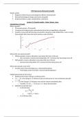
US economy grows ~2% annually
Constant percentage growth represented as linear line on logarithmic scale graph
Growth is concerned with the long-run growth at long time scales (dotted line, x-axis is a long
time period) rather than short term business cycles (red line)
o
Why do We Care about Growth?
Without growth, resource allocation is just about the share of the pie
o Zero sum game: someone becoming better off ⇒ someone else becoming worse off
With growth, resource allocation is also about the size of the pie
o Someone becoming better off ≠ someone else becoming worse off
Where does growth come from?
Growth comes from technology (e.g., Industrial Revolution)
o Technology comes from ideas, research and development
Mathematical tools for the lecture
Models in this lecture will be in continuous time
𝑋𝑡+1 − 𝑋𝑡 is the change in 𝑋 between today and tomorrow (or next month/year/decade)
is the change in 𝑋 between now and the instant immediately after
o Formally, it is (𝑋𝑡+Δ − 𝑋𝑡)/Δ as Δ → 0, hence the derivative
Definitions of growth rates
o In discrete time
o In continuous time
,
(By the chain rule, see appendix for derivation)
The Solow Model
Setup
Distilled from Swan (1956) and Solow (1957)
o Growth exogenously comes from technology and/or population
o Not many knobs or levers are available for policymakers, but still ground-breaking in
showing us where to look for growth
Production function: GDP is produced with three inputs- capital, labour and labour-augmenting
tech
o Monotonicity: If any three inputs increase, GDP increases
o Concavity: Production features diminishing returns for each input
o Constant returns to scale: doubling inputs results in doubling GDP
Industrial interpretation: the following are equivalent
Making one production facility twice as large
Replicating one production facility elsewhere
o The Cobb-Douglas form is mathematically convenient, but not necessary as long as the
properties above hold
o Empirical estimates: 𝛼 is roughly between 0.3 and 0.4
Law of motion of capital: change in capital over time driven by investment and depreciation
(proportional to capital stock level)
o Capital can only be increased by active investment
o Capital can only be decreased by passive depreciation
Existing physical capital cannot be actively reclaimed
Depreciated capital is destroyed: it cannot be reused/recycled
o We assume 𝛿 ∈ (0, 1)
o In Mathematics, this is an Ordinary Differential Equation (ODE)
𝐾𝑡 can be written as 𝐾(𝑡)
K̇ t can be written as 𝐾′(𝑡)
A differential equation involves functions and their derivatives
Solution: a function that satisfies the equation
o Empirical estimates: 𝛿 is about 3% yearly
Investment rule: investment level is a constant fraction (s) of output
, o How exactly savings are directed to investment is not important, we just assume they
are
o The remaining fraction (1 − 𝑠) is spent on consumption
o It can be micro-founded (derived in microeconomics) if intertemporal utility function is
log-additive
o Proportion 𝑠 can be affected by policy (e.g., VAT)
o Important: 𝑠 is the marginal propensity to save, not the average savings rate (here
they’re assumed to coincide)
Resource constraint: GDP is either consumed or invested
o Equivalent to closed economy national accounting, disregarding government spending
o It can be microfounded: equilibrium version of the budget constraint of a household
facing a consumption-savings problem
Population and technology grow at a constant percentage rate per period
o Exogenous and constant net growth rate 𝑔𝐿 and 𝑔𝐴, assumed to be ∈ [0, 1]
o 𝑔𝐿 can be affected by policy (e.g., fertility policies)
o 𝑔𝐴 can be affected by policy (e.g., R&D subsidies, but also see Romer’s model)
o But it does not explain the source of growth
Steady state growth
Naïve definition of steady state: K̇ t =0
o Solving with this definition:
𝐼𝑡 = 𝛿𝐾𝑡 = 𝑠𝑌𝑡.
𝑌𝑡 = 𝛿𝐾𝑡/𝑠 = 𝐾𝑡𝛼(𝐴𝑡𝐿𝑡)1−𝛼.
𝐾𝑡1−𝛼 = (𝑠/𝛿)(𝐴𝑡𝐿𝑡)1−𝛼.
Solution:
o But 𝐴𝑡 and 𝐿𝑡 grow, so K also grows (going against the initial assumption). This violates
the naïve definition of steady state
This model does not have a steady state in physical (and absolute) units
o We need to express variables relative to exogenously growing variables 𝐴𝑡 and 𝐿𝑡
o We focus on 𝑘𝑡:= 𝐾𝑡/(𝐴𝑡𝐿𝑡), i.e., capital per effective unit of labour
o Resulting definition of steady state: k˙ t=0
o Key: 𝐾𝑡 in the steady state will grow matching the pace of 𝐴𝑡 and 𝐿𝑡
o Interpretation: whether 𝐾𝑡 is “big” or “small” depends on tech and population
o Key for some intuition: 𝐾𝑡/𝐿𝑡 known as capital depth (how much capital each worker
uses in production)
Generalised notion of steady-state: achieving time-invariant growth rates in the steady state
o GDP grows at a constant rate driven by 𝑔𝐿 and 𝑔𝐴.
Intensive form of the Solow model
Define 𝑥𝑡 := 𝑋𝑡/(𝐴𝑡𝐿𝑡) for each 𝑋𝑡 ∈ {𝑌𝑡, 𝐼𝑡, 𝐶𝑡, 𝐾𝑡} and rewrite the model
,
o Law of motion:
Derive by solving
Intuitively, 𝑘𝑡 decreases as 𝐴𝑡 and 𝐿𝑡 increases, so you should factor in 𝑔𝐴
and 𝑔𝐿 in addition to depreciation
o The rest of the equations can be easily obtained by dividing both sides by (𝐴𝑡𝐿𝑡)
Steady state: k˙ t=0
o Solving: 𝑖𝑡 = (𝑔𝐴 + 𝑔𝐿 + 𝛿)𝑘𝑡 = 𝑠𝑦𝑡 = 𝑠𝑘𝛼.
o Hence, 𝑠𝑘𝛼 = (𝑔𝐴 + 𝑔𝐿 + 𝛿)𝑘
o In words, investment = “depreciation”
o Rearranging, we obtain:
Phase Diagram and steady state
A phase diagram shows how the state of a dynamical system changes depending on, e.g.,
functional forms and parameter values
Phase Diagram
o
o Vertical axis: y, 𝑐, 𝑖
o Horizontal axis: 𝑘𝑡
o Curves on the graph
The benefits of buying summaries with Stuvia:
Guaranteed quality through customer reviews
Stuvia customers have reviewed more than 700,000 summaries. This how you know that you are buying the best documents.
Quick and easy check-out
You can quickly pay through credit card or Stuvia-credit for the summaries. There is no membership needed.
Focus on what matters
Your fellow students write the study notes themselves, which is why the documents are always reliable and up-to-date. This ensures you quickly get to the core!
Frequently asked questions
What do I get when I buy this document?
You get a PDF, available immediately after your purchase. The purchased document is accessible anytime, anywhere and indefinitely through your profile.
Satisfaction guarantee: how does it work?
Our satisfaction guarantee ensures that you always find a study document that suits you well. You fill out a form, and our customer service team takes care of the rest.
Who am I buying these notes from?
Stuvia is a marketplace, so you are not buying this document from us, but from seller ib45pointer. Stuvia facilitates payment to the seller.
Will I be stuck with a subscription?
No, you only buy these notes for $7.39. You're not tied to anything after your purchase.