Physics for computer science completed assignments, IE University, bachelor of computer science and AI. The four assignments include completed exercises with calculations, formulas and visuals.
Assignment 1: Static fields, Magnetic fields, Electrical fields
Assignment 2: Current, EMF, Magnetic ...
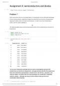
Assignment 4: semiconductors and diodes
In [21]:
from IPython.display import YouTubeVideo
Problem 1
A NTC thermistor, like the one showed below, is a temperature sensor that takes advantage
of how a semiconductor negatively changes its conductivity as a function of temperature.
Suppose we take a piece of certain semiconductor. In order to use it as a temperature
sensor, we first need to calibrate it.
The following table shows experimental measurements of the conductivity as a function of
temperature.
In [2]:
import pandas as pd
import matplotlib.pyplot as plt
import numpy as np
In [3]:
data=pd.read_csv('data_assig.csv')
data
Out[3]: Temperature (K) σ (Ωm)^(-1)
0 620.0 4725.059345
1 560.0 2245.760723
2 510.0 1147.862882
3 480.0 800.000000
4 430.0 481.025258
5 410.0 395.444694
6 330.0 390.507083
7 290.0 382.718994
8 257.0 333.691619
9 232.0 258.023930
10 200.0 168.526251
* a) Use any visualization package that you want to meaningfully represent the
conductivity as a function of temperature, and approximately identify the temperature
intervals in which the semiconductor is found to be in the intrinsic, saturation, and
extrinsic regime. (In Python there are many packages for visualization: matplotlib,
seaborn, pandas... although you may use other software that you feel more
comfortable with).(5 points).
In [30]:
# conductivity as a function of temprature
# plot the graph
plt.scatter(x,y)
plt.plot(x, y_line, "orange")
plt.title("Conductivity as a function of temperature")
plt.xlabel("Temperature (K)")
plt.ylabel("σ (Ωm)^(-1)")
plt.show()
Method 1:
The conductivity of an intrinsic semiconductor increases as the temperature increases. For
an extrinsic semiconductor the conductivity decreases with the increase in temperature,
because the number of majority carriers is almost constant, while the mobility decreases,
which in turn leads to the conductivity decreasing.
Keeping this in mind, while looking at the plotted graph we can approximate the intrinsic
range from 620K to 410K, the saturation regime from 410K to 257K, and the extrinsic regime
from 257K to 200.
Method 2:
The image below shows the intrinsic, saturation, and extrinsic regime when log(σ) is plotted
as a function of 1/T. By plotting log(σ) as a function of 1/T we can compare the data to this
graph.
Los beneficios de comprar resúmenes en Stuvia estan en línea:
Garantiza la calidad de los comentarios
Compradores de Stuvia evaluaron más de 700.000 resúmenes. Así estas seguro que compras los mejores documentos!
Compra fácil y rápido
Puedes pagar rápidamente y en una vez con iDeal, tarjeta de crédito o con tu crédito de Stuvia. Sin tener que hacerte miembro.
Enfócate en lo más importante
Tus compañeros escriben los resúmenes. Por eso tienes la seguridad que tienes un resumen actual y confiable.
Así llegas a la conclusión rapidamente!
Preguntas frecuentes
What do I get when I buy this document?
You get a PDF, available immediately after your purchase. The purchased document is accessible anytime, anywhere and indefinitely through your profile.
100% de satisfacción garantizada: ¿Cómo funciona?
Nuestra garantía de satisfacción le asegura que siempre encontrará un documento de estudio a tu medida. Tu rellenas un formulario y nuestro equipo de atención al cliente se encarga del resto.
Who am I buying this summary from?
Stuvia is a marketplace, so you are not buying this document from us, but from seller beatricemossberg. Stuvia facilitates payment to the seller.
Will I be stuck with a subscription?
No, you only buy this summary for 6,99 €. You're not tied to anything after your purchase.