These notes were prepared based on the lectures and supplemented by information from textbooks and tutorials where parts of the lecture were unclear. Graphs, equations, and bullet-point explanations included. Prepared by a first class Economics and Management student for the FHS Macroeconomics pape...
HT2 Macroecons (Sticky Price Models)
Lecture 4: Inflation bias and monetrary policy
Outline
Use IS-PC-MR model to investigate examples of monetary policy failure (inflation bias)
o Bias refers to equilibrium inflation in excess of optimal inflation target
o Theories developed in late 1970s as possible explanation for sharp upturn in inflation
rates in OECD countries (the Great Inflation discussed in relation to Orphanides’ work)
Reasons for inflation bias and how size of bias relates to
o (i) policy loss function, static vs dynamic
o (ii) expectations assumption, adaptive vs rational
Solutions to inflation bias via institutional reforms such as central bank independence
Can international differences in inflation performance be linked to differences in predicted
inflation bias across countries?
Reasons for Inflation bias
Introduction to inflation bias
Inflation bias can be illustrated in IS-PC-MR with CB's loss function is amended to:
o
o *Careful the distinction between policy maker and CB since it was only after late 20 th
century reforms that CBs became main monetary policy maker
Bliss level of output yT exceeds feasible level ye on VPC
o Could interpret yT > ye as result of policy seeking efficient employment level in presence
of distortions from imperfect competition
Recall ye determined by WS = PS and that employment at that level is sub-
optimal because MPL exceeds opportunity cost of leisure
A social planner seeking to maximise welfare would aim for employment level at
which ES = ED and this corresponds to higher output
o Or yT > ye could be from political cycle
Raising GDP seen as signal of economic competence and a pre-election vote
winner
o Inflation target remains πT (welfare max level)
o MR displaced to the right when yT > ye (Fig 19)
T
Impact of y > ye depends on whether expectations are adaptive or rational and whether loss is
static or dynamic (consider these 4 cases)
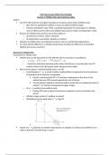
,Equilibrium with Adaptive Expectations (AE), static loss
Suppose economy initially at A in Fig 20 where π e = πT and output in equilibrium on VPC
o This is best feasible point in equilibrium when π = π e required (best point on the VPC line
since it is at inflation target). However, in short-run, PC constraint gives other feasible
points
o CB minimises its loss function by cutting r and raising output and inflation to B on MR
o Under adaptive expectations, PC shifts up as next period π e = πB
o Policy-maker deviates to C through again setting r < r s
o Process repeats until Z reached and there is no incentive for further deviations
Z is a stable equilibrium point since it is on both VPC (feasible) and MR (best
response of policy maker)
Marginal cost of inflation is 2βπ in loss (the partial derivative of the loss
function)
At A, the marginal cost of increased inflation is outweighed by the benefit of
increasing output, so output is closer to y T (there is an incentive for deviation by
policy maker)
At Z, the marginal cost of inflation is sufficiently high to offset benefit of higher
output (no incentive for deviation)
Equilibrium inflation exceeds efficient target level and (π Z – πT) is inflation bias
Factors affecting the magnitude of the inflation bias
o Larger (yT – ye), MR line displaced further right, and its intersection with VPC will be
higher, so inflation bias would be larger.
o The steeper the MR line (small α and β), the higher the intersection with VPC, and the
larger the inflation bias.
Intuition: smaller α (PC curve slope), smaller inflation cost of output increase, so
policy makers choose to go closer to yT more aggressively, increasing the
equilibrium inflation bias
Intuition: smaller β (policy maker inflation aversion), policy maker is more
accepting of higher inflation (cost of pursuing yT), pursues yT more aggressively,
increasing the equilibrium inflation bias
Equilibrium with Adaptive Expectations (AE), dynamic loss
, Under dynamic loss, CB aims to minimise
Starting at A in Fig 20, deviation to B reduces current loss by (L A – LB) where LA is the value of loss
function on contour through A (it must have reduced current loss since static loss function policy
maker pursues it)
o But next period outcome at C has LC > LA. It is worse than if there had been no deviation
from A
o The same is true in all future periods. Per period loss relative to no deviation rises and
peaks at (LZ – LA)
o Policy expansion from A implies one-off gain for infinite sequence of losses
o When δ → ∞ (in the case of static losses), CB deviates from A and ends up at Z
o But for the other polar case of δ = 0, never deviate from A (infinite losses ahead are
never worth it)
o Intermediate values of δ imply excess inflation but less than full inflation bias at Z
Initial correction is somewhere between A and B
Factors affecting the magnitude of the inflation bias
o The smaller δ is (more patient policy maker), the closer the final point is to A, and the
lower the inflation bias
Equilibrium with Rational Expectations
Given rational inflation expectations, the only output/ inflation outcome that can occur is Z
o Any other expected inflation is irrational as CB would deviate and produce a different
inflation level
o It is only at πe = πZ that policy is in line with actual inflation rate
o So, points A, B, C (considered under AE) are not observed under RE
Inflation bias at Z still occurs under dynamic loss irrespective of δ
o Under AE, there was a clear link between periods (setting low inflation today yields low
inflation expectations tomorrow), so dynamic loss function CB does not raise output
fully to B to reduce losses in future periods
This was the basis for establishing an equilibrium on VPC at π < π Z given a
dynamic loss function with finite δ
o Under RE, there is nothing to connect periods
There is no incentive to raise inflation lower than B due to dynamic loss function
Own thoughts: since there is no C and other points moving slowly to Z under RE,
there is no incentive for CB to increase output by less than point B, even with
dynamic loss. So, the CB with dynamic loss has incentives to deviate to B.
o If CB announces today that it will set π A, this will not induce low expected inflation
tomorrow since the private sector knows that if it sets π e = πA, tomorrow the CB will
deviate to B (not halfway despite dynamic loss function) leading to higher actual
inflation
o A similar deviation argument applies for any π e < πZ that might be set tomorrow
o Hence, πe = πZ is inescapable tomorrow
o Knowing this, CB does not have any incentive to set π A today, or any π < πZ.
Hence, for RE, inflation bias is at Z regardless of static or dynamic loss function of CB
Los beneficios de comprar resúmenes en Stuvia estan en línea:
Garantiza la calidad de los comentarios
Compradores de Stuvia evaluaron más de 700.000 resúmenes. Así estas seguro que compras los mejores documentos!
Compra fácil y rápido
Puedes pagar rápidamente y en una vez con iDeal, tarjeta de crédito o con tu crédito de Stuvia. Sin tener que hacerte miembro.
Enfócate en lo más importante
Tus compañeros escriben los resúmenes. Por eso tienes la seguridad que tienes un resumen actual y confiable.
Así llegas a la conclusión rapidamente!
Preguntas frecuentes
What do I get when I buy this document?
You get a PDF, available immediately after your purchase. The purchased document is accessible anytime, anywhere and indefinitely through your profile.
100% de satisfacción garantizada: ¿Cómo funciona?
Nuestra garantía de satisfacción le asegura que siempre encontrará un documento de estudio a tu medida. Tu rellenas un formulario y nuestro equipo de atención al cliente se encarga del resto.
Who am I buying this summary from?
Stuvia is a marketplace, so you are not buying this document from us, but from seller ib45pointer. Stuvia facilitates payment to the seller.
Will I be stuck with a subscription?
No, you only buy this summary for $7.39. You're not tied to anything after your purchase.