This document contains all the notes from the synchronous and asynchronous lectures throughout the year and is split up lecture by lecture. This document on its own, is sufficient to get a top mark in your end of year exam for EC345 Behavioural Economics.
What is Behavioural Economics? A method of economic analysis that applies psychological
insights into human behaviour to explain economic decision making. It gained momentum in
the 1950s as it was easier to target standard economic theory.
Neoclassical economics take a normative approach and adopts basic axioms of rationality
which can be described by a standard utility function that is only observable from choices
and is therefore ordinal in nature.
Week 2: Decision Under Uncertainty: Expected Utility Theory:
We look at uncertainty: Suppose there are a number of uncertain outcomes, or lotteries. We
want to represent preferences over different outcomes.
Expected Utility Theory: If someone’s preferences can be represented by an expected utility
function, all we need to pin down their preferences over uncertain outcomes are their
payoffs from the certain outcomes.
Expected Utility Theory (Axioms):
There are four required axioms:
1. Completeness: it is always possible to rank possible outcomes, even if they are equal
2. Transitivity: If X >Y ,∧Y >Z , then X > Z
Preferences are consistent
Preferences are rational if transitivity and completeness are satisfied
3. Continuity: If X > Y > Z, then the agent is indifferent between Y and some weighted
average of X and Z
4. Independence: if we have 3 lotteries and we prefer X > Y, adding a third lottery Z will
not change this preference, i.e. mixing a third lottery does not affect preference over
first 2
If all 4 axioms are met, then it is possible to assign a real utility to each outcome by
multiplying the probability of each outcome by the utility from this outcome and adding
these up. Such that:
X ≥ Y if and only if U ( X ) ≥U (Y )
Example: Consumer has £10 and contemplates a gamble with 50% chance of winning £5 and
50% chance of losing £5
Expected value of wealth is 0.5 ( 5 ) +0.5 ( 15 ) =£ 10
Expected utility of wealth is 0.5∗u ( 5 ) +0.5∗u(15)
For a risk averse consumer, the utility of expected value of wealth, u(10) is greater than the
expected utility of wealth, 0.5∗u ( 5 ) +0.5∗u(15). Concave utility function.
Anomalies/Deviations from the Expected Utility Theory: Allais (1953) Paradox:
Gamble A Gamble B Gamble C Gamble D
100% chance of winning 5 89% chance of winning 5 million 11% chance of 10% chance of winning
million winning 5 million 15 million
1% chance of winning nothing 89% chance of 90% chance of winning
winning nothing nothing
10% chance of winning 15
million
,Most people choose Gamble A vs Gamble B and Gamble D vs Gamble C
Gamble A vs B depends on a person’s preferences for risk
This is not consistent with EUT -> violation of independence axiom
If you choose Gamble A you should choose Gamble C.
u ( A ) >u(B) for most people:
0.89 u ( 5 million ) +0.11 ( 5 million ) >0.89 u ( 5 million ) +0.1 u ( 15 million ) +0.01 u(0)
0.11 u ( 5 million ) >0.1 u ( 15 million ) +0.01 u ( 0 ) … eq( i)
In second pair wise choice, most people chose gamble D over gamble C. So, u ( D ) >u(C )
0.1 u ( 15 million ) +0.89 u ( 0 ) +0.01 u ( 0 ) >0.11 u ( 5 million ) +0.89 u(0)
0.1 u ( 15 million ) +0.01 u ( 0 ) >0.11 u ( 5 million ) … eq(ii)
Eq(i) and eq(ii) directly contradict each other which shows why Allais Paradox violates the
independence axiom.
Allais (1953) Paradox – violation of independence axiom to minimise risk (i.e. prefer
certainty over risky outcome of 0 in gamble A) – avoidance of potential disappointment
(Loomed & Sugden, 1986)
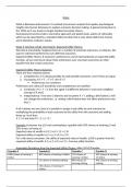
Ellsberg Paradox: Imagine an urn contains 90 balls from which 30 are known to be red and
the remaining 60 are either blue or yellow. One ball is to be drawn at random from the urn.
Choose between the following gambles:
Gamble A: - $100 if the ball is red, nothing otherwise
Gamble B: - $100 if the ball is blue, nothing otherwise
And one between the following:
Gamble C: -$100 if the ball is red or yellow, nothing otherwise
Gamble D: - $100 if the ball is blue or yellow, nothing otherwise
30 balls 60 balls
Gamble Red Blue Yellow
A $100 $0 $0
B $0 $100 $0
C $100 $0 $100
D $0 $100 $100
EUT predicts that if individuals choose A, they should choose C
You will only choose A over B if you think probability of red balls is higher than probability of
blue balls
This implies you should choose C (prob of red + yellow) over D (prob of blue +
yellow)
In reality most people choose A over B and D over C. Violates the independence axiom
Explaining the behaviour: A > B because the proportion of red balls is known and D > C
because the proportion of blue and yellow balls is known
It is thought that betting for or against the known information (red ball) is safer than
betting for or against the unknown (blue ball)
Ellsberg (1961) explains these in terms of people’s dislike for ambiguity, or ambiguity
aversion.
Ambiguity can be defined as uncertainty about probability created by missing information
that is relevant and could be known.
,Framing Effect: The following experiment is an all-time-classic brought forward by Amos
Tversky and Daniel Kahneman (1986)
Imagine that the U.S. is preparing for the outbreak of an unusual Asian disease, which is
expected to kill 600 people. Two alternative programs to combat the disease have been
proposed and you have to choose one of them. Assume that the exact scientific estimates of
the consequences of the programs are as follows:
600 lives are threatened: Action (A) saves 200 lives; Action (B) saves all 600 lives with
probability 1/3 and saves nobody with probability 2/3.
600 lives are threatened: Action (C) causes 400 to die with probability 1/3; Action (D) causes
600 to die with probability 2/3 and causes nobody to die with probability 1/3
The majority picked action A even though action B saves more lives. The majority picked
action D over action C
These problems are identical, apart from how they are framed. Yet, the most common
choices are different. The way we make choices also depends on the way in which they are
presented to us!
Prospect Theory: The value of a prospect V, is expressed in terms of two scales:
The value function v(x) and the weighting function π ( p)
V assigns to each outcome x a number v(x), which reflects the subjective outcome.
π associates with each probability p a decision weight π ( p), which reflects the impact of the
probability on the overall value of the prospect.
If ( x , p ; y , q ) is a regular prospect, then: V ( x , p ; y , q )=π ( p ) v ( x ) + π ( q ) v ( y)
Compare this to the expected utility of a prospect: U =pu ( x ) +qu( y)
Prospect Theory – Value Function: is S-shaped due to three main principles:
Reference dependence – outcomes are viewed relative to a reference point and
hence coded as gains or losses; Diminishing sensitivity – changes in value have a
greater impact near the reference point than away from the reference point;
Loss aversion – pain from losses has stronger effect than pleasure from gains.
Hence, concave in gains domain, convex in losses domain (risk seeking). Notice losses
domain is steeper also (loss aversion!).
Prospect Theory – Weighting Function: is convex due to two main principles:
Reference dependence and diminishing sensitivity.
Reference point is the 0 point which is the impossibility point and 1 which is the
certainty point. What people do is the solid black line due to reference
dependence. They overweight very low probabilities and underweight very high
probabilities.
Diminishing sensitivity -> as we move away from 0% and 100% we become less
sensitive to changes in probability
A typical weighting function is concave for small probabilities (above 45 degree
line) and convex for medium to large probabilities (below 45 degree line)
Empirical Applications: Endowment Effect: The value that an individual assigns to an object
appears to increase substantially as soon as that individual is given the object.
, This is contrary to standard economic theory; preferences are not independent of
entitlements, but instead depend on their reference positions.
Kahneman, Knetsch & Thaler (1990) experimentally proved the endowment effect.
In the experiments, individuals were endowed with a mug, or with the money to buy this
mug. Their WTP and WTA are elicited: Willingness to Pay is max price an individual is willing
to pay to get a good; Willingness to Accept is minimum compensation demanded by an
owner to sell a good. Standard assumption imply that WTA = WTP
They found that WTA > WTP.
Thaler (1980) labelled this increased value of a good as the endowment effect. The effect is
a manifestation of loss aversion. An implication of this asymmetry is that if a good is
evaluated as a loss when it is given up and as a gain when it is acquired, loss aversion will,
on average, induce a higher dollar value for owners than for potential buyers
Equity Premium Puzzle: Stocks or equities tend to have more variable annual price changes
(or returns) than bonds do
As such, the average return to stocks is higher, as a way of compensating investors
for the additional risk they bear
Stock returns were about 8% per year higher than bond returns. The equity premium
should instead actually be around 0.35%
Mehra and Prescott (1985) showed that under the standard assumptions of economic
theory, investors must be extremely risk-averse to demand such a high premium
Bernartzi and Thaler (1997): myopic loss aversion theory: Investors are not just averse to the
variability of returns, they are averse to loss (the chance that returns are negative).
Annual stock returns are negative much more frequently than annual bond returns and so a
large equity premium is demanded as compensation.
In long term, return from stocks is higher than bonds, so this means investors must be
extremely short-sighted over a short horizon. Hence, the equity premium puzzle can be
explained by loss aversion and a short evaluation period.
Two factors contribute to an investor being unwilling to bear the risks associated with
holding equities, loss aversion and a short evaluation period – myopic loss aversion
The Disposition Effect: is the tendency of investors to hold losing investments too long and
sell winning investments too soon.
Disposition effect is anomalous because the purchase price of a stock should not matter, but
people are comparing it to a reference point instead (their purchase price)
If you think the stock will rise, you should keep it; if you think it will fall, you should
sell it
Realised gains are shares that have been sold for a profit
Realised losses are shares sold for losses
Paper gains/losses are shares that are in profit/loss but have not been sold yet.
realised losses
Proportion of losses realised: PLR =
realised losses+ paper losses
Les avantages d'acheter des résumés chez Stuvia:
Qualité garantie par les avis des clients
Les clients de Stuvia ont évalués plus de 700 000 résumés. C'est comme ça que vous savez que vous achetez les meilleurs documents.
L’achat facile et rapide
Vous pouvez payer rapidement avec iDeal, carte de crédit ou Stuvia-crédit pour les résumés. Il n'y a pas d'adhésion nécessaire.
Focus sur l’essentiel
Vos camarades écrivent eux-mêmes les notes d’étude, c’est pourquoi les documents sont toujours fiables et à jour. Cela garantit que vous arrivez rapidement au coeur du matériel.
Foire aux questions
Qu'est-ce que j'obtiens en achetant ce document ?
Vous obtenez un PDF, disponible immédiatement après votre achat. Le document acheté est accessible à tout moment, n'importe où et indéfiniment via votre profil.
Garantie de remboursement : comment ça marche ?
Notre garantie de satisfaction garantit que vous trouverez toujours un document d'étude qui vous convient. Vous remplissez un formulaire et notre équipe du service client s'occupe du reste.
Auprès de qui est-ce que j'achète ce résumé ?
Stuvia est une place de marché. Alors, vous n'achetez donc pas ce document chez nous, mais auprès du vendeur bspurs11. Stuvia facilite les paiements au vendeur.
Est-ce que j'aurai un abonnement?
Non, vous n'achetez ce résumé que pour €23,44. Vous n'êtes lié à rien après votre achat.