Summary Notes for Economic Growth and Institutions (Tilburg Univeristy)
34 vues 3 fois vendu
Cours
Economic Growth and Institutions (30L207B6)
Établissement
Tilburg University (UVT)
The summary is based off ALL video lectures, slides, and readings. All derivations or time graphs that you need to know, and other concepts such as Romer model, Malthusian equilibrium, etc are in this summary. Knowing the material in this summary will allow one to confidently enter the exam and ach...
The purpose of this document is to attempt to embody the key aspects of each chapter studied,
highlight certain parts that the book or professor highlighted and to keep it as concise as
possible. Hence, we will not go into many examples, just the theory. Examples can be found in
the book, slides/lectures, or online. I will attempt to keep each summary within 2-3 pages, but if
a chapter is too large, this may not be possible. Feel free to use the table of contents to the left
to scroll through quicker.
Week One:
This week is an introduction (Lecture 1) and the basics to growth rates and solow model
(Lecture 2)
Lecture 1:
The first lecture looks at some basic facts about economic growth. It looks at the things we can
measure (GDPpc in current prices and in constant prices & GDPpc PPP in current prices and in
constant prices). What we can compare is the average income of a country over time. Let’s look
at some facts:
(1) There is an enormous difference in income levels across countries
today.
(2) GDPpc V GDP per worker
GDP per worker usually is seen as a productivity measure rather than
welfare. But it can be used for welfare. We will not differentiate in this
course because we assume population = workers because it is a long
run model, we assume 0 unemployment.
Note: On the slides you can see a cool graph about the cumulative distribution of world
population by GDP per worker, the long vertical parts is a large country like China or India and
the long horizontal parts are a bunch of small countries with similar GDP per worker.
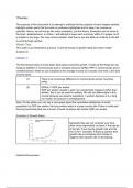
Evolution of Growth Rates:
Generally they are not constant over time,
often more exponential, as seen in the picture
to the left. If you log the growth rate and the
line is flat = constant, if slope is positive then
growth rate is increasing and if slope is
negative then growth rate is decreasing.
Industrial Economies:
, 𝐾
(1) The ratio of capital to output has been stable ⇒ 𝑌
𝐾
(2) Capital per worker has grown at a sustained rate (G) ⇒ 𝐿
𝑔↑
𝐾
(b) Output per worker has grown at sustained rate ⇒ since 𝐿
𝑔 ↑, and
𝑌 𝐾/𝐿 𝐿 𝑌
𝐿
= 𝐿/𝐿 𝐿
, 𝐿
grows at g too!
(3) Capital and labor have captured stable shares of national income
𝑊𝐿 𝑊 𝑌
(a) Wages have grown at a sustained rate: α𝐿 = 𝑌
= 𝑔↑ 𝑌/𝐿
(since 𝐿
grows at
rate g, so much W because the whole thing grows at a sustained rate!
𝑅𝐾 𝑅
(b) The real interest rate, or return to capital has been stable: α𝐾 = 𝑌
=
(𝑌/𝐾)
Lecture 2:
This lecture focuses more on the Solow Growth Model. Note: There is a lot of math and
derivations, it is good to take some time to understand it all!
Solow Growth Model:
Part I: Physical Capital (K)
→ Infrastructure and machinery. It is productive and can be produced, it is rival in
its nature, it earns a return (incentives to invest in it) and it depreciates. There is also a positive
relationship between capital (K) and output (Y).
Production Function: 𝑌(𝑡) = 𝐹(𝐾(𝑡), 𝐿(𝑡))
Assumption 1) constant returns to scale for any λ > 0 in λ𝑌(𝑡) = 𝐹(λ𝐾(𝑡), λ𝐿(𝑡))
In per worker terms:
𝑌(𝑡) 𝐾(𝑡) 𝐾(𝑡) 1
𝐿(𝑡)
= 𝐹( 𝐿(𝑡)
, 1) = 𝑓( 𝐿(𝑡)
). Here we see that λ = 𝐿
Assumption 2) Diminishing marginal returns
*Profit maximization and return to inputs.
These two assumptions, together with the assumption that there are a large number of
homogenous firms (so price-taking): we get the representative firm. We can model this firm with
one simple function, often the Cobb-Douglas production function.
Cobb-Douglas Production Function:
α 1−α
𝑌(𝑡) = 𝐾(𝑡) 𝐿(𝑡)
Satisfies A1 and A2
Properties:
- Constant elasticity of output wrt each factor of production (K and L)
- Constant factor income shares (in line with stylized facts - Lecture 1)
α α−1
𝑀𝑃𝐿: 𝑤 = (1 − α)(𝐾/𝐿) & 𝑀𝑃𝐾: 𝑅 = 𝑎(𝑘/𝐿)
Two Main Equations for Solow Model:
, α 1−α
𝑌(𝑡) = 𝐾(𝑡) 𝐿(𝑡) Eq1
And
𝐾 * (𝑡) = 𝑠𝑌(𝑡) − δ𝐾(𝑡) Eq2
Capital Accumulation (s = savings/investment rate ∈ (0, 1) so sY = gross investment
A large step is how do we derive Eq2? This will be done here:
We assume a closed economy w/out government, hence 𝑌(𝑡) = 𝐶(𝑡) + 𝐼(𝑡) Eq3
•
Gross investment and capital accumulation: 𝐼(𝑡) = 𝐾 (𝑡) + δ𝐾(𝑡) Eq4
•
𝐾 (𝑡) is the derivative of K(t)
Our basic Macro identity (𝑌 = 𝐶 + 𝑆) is going to be important. With this identity we are able to
do the following:
Firstly, we assume that savings/investment rate (s) is constant, hence:
𝑆(𝑡) = 𝑠𝑌(𝑡) → 𝐶(𝑡) = (1 − 𝑠)𝑌(𝑡); 𝐼(𝑡) = 𝑠𝑌(𝑡) Eq5
Combining Eq3-Eq5 we are able to obtain Eq2!
Expressing Eq1 & Eq2 in per Capita Terms:
𝑌(𝑡) 𝐾(𝑡) α 𝐿(𝑡) 1−α α
Total Output: 𝑦(𝑡) = 𝐿(𝑡)
=[ 𝐿(𝑡)
] [ 𝐿(𝑡) ] = 𝑘(𝑡)
In the steady state, the change in K is zero,
hence we can simply graph the two lines you
see to find it. It is always important to know
this! If we utilize this, to find, let’s say the
steady state value of k, we get:
Les avantages d'acheter des résumés chez Stuvia:
Qualité garantie par les avis des clients
Les clients de Stuvia ont évalués plus de 700 000 résumés. C'est comme ça que vous savez que vous achetez les meilleurs documents.
L’achat facile et rapide
Vous pouvez payer rapidement avec iDeal, carte de crédit ou Stuvia-crédit pour les résumés. Il n'y a pas d'adhésion nécessaire.
Focus sur l’essentiel
Vos camarades écrivent eux-mêmes les notes d’étude, c’est pourquoi les documents sont toujours fiables et à jour. Cela garantit que vous arrivez rapidement au coeur du matériel.
Foire aux questions
Qu'est-ce que j'obtiens en achetant ce document ?
Vous obtenez un PDF, disponible immédiatement après votre achat. Le document acheté est accessible à tout moment, n'importe où et indéfiniment via votre profil.
Garantie de remboursement : comment ça marche ?
Notre garantie de satisfaction garantit que vous trouverez toujours un document d'étude qui vous convient. Vous remplissez un formulaire et notre équipe du service client s'occupe du reste.
Auprès de qui est-ce que j'achète ce résumé ?
Stuvia est une place de marché. Alors, vous n'achetez donc pas ce document chez nous, mais auprès du vendeur mathieuvandevel. Stuvia facilite les paiements au vendeur.
Est-ce que j'aurai un abonnement?
Non, vous n'achetez ce résumé que pour €7,96. Vous n'êtes lié à rien après votre achat.