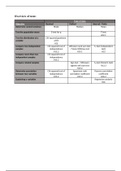
Overview of tests:
Type of data
Objective Nominal Ordinal Interval / Ratio
Determine central tendency Mode Median Mean
Test the population mean Z-test for p T-test
H12.1
Test the distribution of a Chi-squared goodness-
variable of-fit
H15
Compare two independent Chi-squared test of Wilcoxon rank sum test T2-test (independent
samples independence / Mann-Whitney test test)
H15.2 H19.1 H13
Compare more than two Chi-squared test of
independent samples independence
H15.2
Compare related samples Sign test / Wilcoxon TD-test (Paired t-test)
signed rank sum test H13.3
H19.2
Determine association Chi-squared test of Spearman rank Pearson correlation
between two variables independence correlation coefficient coefficient
H15.2 H19.3 H16.4
Explaining a variables Regression analysis
H16
,Normal Distributed
Z-test and estimator of p F-test (to perform before 2T-Test)
Test to determine whether two population Tests the equality of variances (using sample)
means are different when the variance are Datatype: interval
known and the sample size is large.
Using population data 2T-Test (independent)
Z-test (proportion) Tests if two population means are equal
Datatype: nominal Datatype: interval
Use F-test first to know whether to use the
T-test and estimator of µ equal or unequal variance test
Test to determine whether two population
means are different when the variance are
Paired sample T-test (same but matched
unknown. Descriptive measurement: central
pairs)
location. Using sample data
Datatype: interval / ratio
Chi-squared contingency table
Test whether
Chi-squared there is a difference
goodness-of-fit test / relationship
between
Tests expected
whether there isfrequencies
a differenceinbetween
one or more
categories
expected frequencies in one or more
Datatype: nominal
categories.
Datatype: interval
Regression analysis
Test relationship between one or more
variables
Datatype: interval
Nonnormally Distributed
Wilcoxon Rank Sum Test Wilcoxon Signed Rank Sum Test
Tests whether population distribution are Tests for consistent difference between pairs of
identical or not (whether entire populations observations. Compare two populations
differ on themselves). Compare two Datatype: interval
populations Matched pairs
Datatype: interval, ordinal
Independent samples Sign Test
Tests for consistent difference between pairs of
Spearman Rank Correlation Coefficient observations. Compare two populations
Test relationship between two variables Datatype: ordinal
Datatype: ordinal or interval. Matched pairs
Independent samples
Pearson Correlation Coefficient
Test relationship between two variables
Datatype: ONLY interval
Independent samples
If there is an ordinal variable; the population
is nonnormal and therefore we should use the
Spearman Rank Correlation Coefficient.
,Nominal: unranked categories; eye colour, gender etc (p. 15)
Ordinal: ranked categories; exam grade, satisfaction level (p. 14)
Interval: real numbers; time, height, weight, income (p. 15)
Ratio: variables always have a zero point
Inferential statistics: doing calculations with statistics (p.3)
Descriptive statistics: mean, median, mode, variance (p.2)
Sample statistics: s, p, p har etc.
Sample space: list all possible outcomes of a random experiment. An individual outcome is a simple event
(p. 175)
Sample inference: process of estimating, predicting or decisioning about a population based on sample data
(p. 5).
Parameter: descriptive measure of a population (p.5)
Statistic: descriptive measure of a sample (p.5).
Population statistics: ơ, µ
P-value: largest at which the null hypothesis can be rejected
Discrete random variable: countable number of values (p. 215)
Continuous random variable: uncountable e.g. time (p. 215)
Mean: summing all observations and divide by number of observations (p. 99)
Median: place all observations in order, median is the middle (p. 100)
Mode: the observation that occurs with the greatest frequency (p. 101).
Type I error: reject true H0 (null hypothesis) (p.355)
Type II error: not rejecting false H0 (null hypothesis) (p.355)
Unbiased estimator: an estimate who’s expected value is equal to that parameter
Measures of variability: range, variance, standard deviation
Coefficient of determination: SSR / SSE + SSR
Range: largest observation – smallest observation (p. 108)
Variance: related to standard deviation, first calculate variance (s 2 is sample, ơ2 population variance)(p.108)
Standard deviation: square root the variance = standard deviation (p. 112) question 4.22
Empirical rule: histogram bell-shaped? Standard deviation tells how many observations. Use rule (p. 113)
Chebysheff’s Theorem: same as empirical rule but applies to all histograms. Follow formula (p. 114)
Bar chart: displays frequencies; nominal data (p. 19)
Pie chart: displays relative frequencies; nominal data (p.19)
Cross-classification table: describe relationship between two nominal variables; list frequencies of each
combination of the values of the two variables (p. 33)
Number of classes Histogram: Table 3.2 (p. 49)
Class Interval Widths: largest observation – smallest observation / number of classes (p. 49)
Positively skewed: histogram with a long tail extending to the right (p. 50)
Negatively skewed: histogram with a long tail extending to the left (p. 50)
Modal class: class with largest number of observations (p. 50)
Unimodal histogram: one with single peak (p. 50)
Bimodal histogram: one with two peaks, not necessarily equal in height (p. 51)
Bell shape histogram: symmetric unimodal histogram (p. 51)
Stem-and-leaf display: split observations into stem and leaf, list stems in order, list leaves in order.
Histogram turned on its side (p. 57)
Ogive: a cumulative relative frequency distribution in graphical form (p. 59/60)
Frequency distribution: lists all number of observations that fall into each class interval.
Relative frequency distribution: dividing the frequencies by number of observations
Scatter diagram: list dependent variable (Y) and independent variable (X) (p. 75)
Coefficient of Variation: measure of variability, set of observations is the standard deviation / mean (p. 115)
, Coefficient of Correlation: numerical measures of linear relationship, tells us the strength of the relationship
(p.128)
Coefficient of Determination: most extensive method for measuring a linear relationship (p. 139)
Least Squares Method: objective method of producing a straight line in the scatter diagram (p. 132)
Joint probability: the intersection of events A and B is the event that occurs when both A and B occur
(p. 179)
Conditional probability: the probability of one event given the occurrence of another related event (p. 182)
Percentile: is the value for which P percent are less than that value and (100-P)% are greater than that value
(p.117)
Location of a Percentile: Lp = (n + 1)(P / 100) (p. 118)
Interquartile range: Q3 – Q1 measures the spread of the middle 50% of the observations. (p. 120)
Box plot: lists minimum and maximum observations and the first, second and third quartiles. (p. 120)
Covariance: numerical measures of linear relationship; only measures the direction of the relationship (p. 127)
Addition rule (probability): calculate the probability of the union of two events (p. 191).
Bivariate distribution: provides probabilities of combinations of two variables (p. 225)
Binomial Probability Distribution: probability of x successes (p) in a binomial experiment with n trials
(p. 241)
Poisson Distribution: Binomial is about number of trials, Poisson is about interval of time of specific region
(p.247)
Central Limit Theorem: The larger the sample size, the more closely the sampling distribution of X̄ will
resemble a normal distribution (p. 306)
Rejection region: range of values, if the test statistic falls into that range we reject the null hypothesis (p. 360).
p-Value: test whether the null hypothesis should be rejected or not rejected (p. 363/364).
One-tail test: rejection region is located in only one tail of the sampling distribution (p. 370)
Two-tail test: rejection region is located on both tails of the sampling distribution (p. 371)
Pooled variance estimator: weighted average of the two sample variances with the number of degrees of
freedom (p.443)
Equal-variances t-test: when the two populations are normal (p. 443)
Unequal-variance t-test: if the sampling distribution is neither normal nor Student t distributed. (p. 444)
Multinomial experiment: Binomial 2 outcomes exist (success, fail), multinomial ≥ 2 possible outcomes per
trial (p.577)
Rule of Five: expected values should be at least 5 to ensure that the chi-squared distribution provides an
adequate approximation of the sampling distribution (p. 590)
Outlier: observation that is unusually small or unusually large (p.650)
Error variable: the error accounts for all the variables, measurable and immeasurable that are not part of the
model.
Residuals: deviations between actual data points and the line (denoted as e i) (p. 613)
Les avantages d'acheter des résumés chez Stuvia:
Qualité garantie par les avis des clients
Les clients de Stuvia ont évalués plus de 700 000 résumés. C'est comme ça que vous savez que vous achetez les meilleurs documents.
L’achat facile et rapide
Vous pouvez payer rapidement avec iDeal, carte de crédit ou Stuvia-crédit pour les résumés. Il n'y a pas d'adhésion nécessaire.
Focus sur l’essentiel
Vos camarades écrivent eux-mêmes les notes d’étude, c’est pourquoi les documents sont toujours fiables et à jour. Cela garantit que vous arrivez rapidement au coeur du matériel.
Foire aux questions
Qu'est-ce que j'obtiens en achetant ce document ?
Vous obtenez un PDF, disponible immédiatement après votre achat. Le document acheté est accessible à tout moment, n'importe où et indéfiniment via votre profil.
Garantie de remboursement : comment ça marche ?
Notre garantie de satisfaction garantit que vous trouverez toujours un document d'étude qui vous convient. Vous remplissez un formulaire et notre équipe du service client s'occupe du reste.
Auprès de qui est-ce que j'achète ce résumé ?
Stuvia est une place de marché. Alors, vous n'achetez donc pas ce document chez nous, mais auprès du vendeur nikkinuman. Stuvia facilite les paiements au vendeur.
Est-ce que j'aurai un abonnement?
Non, vous n'achetez ce résumé que pour €4,99. Vous n'êtes lié à rien après votre achat.