Statistics 2
Basic commands in SPSS
Data view: help us visualize data as an excel sheet where we can work on the
variables
Variable view: helps us change different aspects of our variables
1. Graphs (any kind): Graphs → Legacy dialogs → Choose the type here
2. Covariance & Correlation: Analyze → Correlate → Bivariate → Options
→ cross-product deviations & covariances
3. Compute a new variable: Transform → Compute variable
4. Summary statistics: Analyze → Descriptive statistics → Frequencies
→ Statistics → Display frequency tables
Chapter 5
We use three tools to determine the relationship:
Scatter plots: to determine the type of relationship between X and Y
Covariance and correlation coefficient: to determine the degree of linear relationship
Regression line: to understand how Y depends on X (Y is a dependent variable,
while X is an independent variable)
Scatter plot
graphical interpretation of the relationship between 2 variables, an independent one
(called X by convention) and a dependent one (called Y by convention).
Click graphs → legacy dialogs → scatter plots → simple scatter
Covariance and correlation coefficient
Covariance (cov) = measure of the joint variability of 2 variables. It indicates the
direction of the linear relationship (negative or positive).
Correlation coefficient (corr) = measures mainly the strength of the linear
relationship between the 2 variables (strong/weak correlation)
don’t have to learn these by heart.
When analyzing data, we will mostly use the correlation because covariance
includes the scaling of variables (it influences the results).
Corr is dimensionless and varies between -1<corr<1
, Correlation cases
1. Corr = + → X and Y are positively related (can be weak or strong)
2. Corr = - → X and Y are negatively related (can be weak or strong)
3. Corr = 1 → Perfect positive linear relationship
4. Corr = -1 → Perfect negative linear relationship
5. Corr = 0 → X and Y are uncorrelated
In SPSS
1. Open SPSS
2. Go to analyze → Correlate → Bivariate and drag the variables into
the box.
3. Options → Cross product deviations and covariances and exclude
cases pairwise
4. Click Continue, then OK and run the program.
Sometimes, X and Y may be strongly related, but in a nonlinear way!
In order to avoid making mistakes, we will use the linear regression to represent X
and Y.
Simple linear regression
SLRM is a linear approach to modeling the relationship between two variables.
SLRM: Y is a linear function of X (Y is dependent on X)
The regression line is the line on the graph that best fits the population of points.
“Best” entails that the sum of the squared errors is minimized (close to 0).
Let’s understand what coefficients do!
Basic commands in SPSS
Data view: help us visualize data as an excel sheet where we can work on the
variables
Variable view: helps us change different aspects of our variables
1. Graphs (any kind): Graphs → Legacy dialogs → Choose the type here
2. Covariance & Correlation: Analyze → Correlate → Bivariate → Options
→ cross-product deviations & covariances
3. Compute a new variable: Transform → Compute variable
4. Summary statistics: Analyze → Descriptive statistics → Frequencies
→ Statistics → Display frequency tables
Chapter 5
We use three tools to determine the relationship:
Scatter plots: to determine the type of relationship between X and Y
Covariance and correlation coefficient: to determine the degree of linear relationship
Regression line: to understand how Y depends on X (Y is a dependent variable,
while X is an independent variable)
Scatter plot
graphical interpretation of the relationship between 2 variables, an independent one
(called X by convention) and a dependent one (called Y by convention).
Click graphs → legacy dialogs → scatter plots → simple scatter
Covariance and correlation coefficient
Covariance (cov) = measure of the joint variability of 2 variables. It indicates the
direction of the linear relationship (negative or positive).
Correlation coefficient (corr) = measures mainly the strength of the linear
relationship between the 2 variables (strong/weak correlation)
don’t have to learn these by heart.
When analyzing data, we will mostly use the correlation because covariance
includes the scaling of variables (it influences the results).
Corr is dimensionless and varies between -1<corr<1
, Correlation cases
1. Corr = + → X and Y are positively related (can be weak or strong)
2. Corr = - → X and Y are negatively related (can be weak or strong)
3. Corr = 1 → Perfect positive linear relationship
4. Corr = -1 → Perfect negative linear relationship
5. Corr = 0 → X and Y are uncorrelated
In SPSS
1. Open SPSS
2. Go to analyze → Correlate → Bivariate and drag the variables into
the box.
3. Options → Cross product deviations and covariances and exclude
cases pairwise
4. Click Continue, then OK and run the program.
Sometimes, X and Y may be strongly related, but in a nonlinear way!
In order to avoid making mistakes, we will use the linear regression to represent X
and Y.
Simple linear regression
SLRM is a linear approach to modeling the relationship between two variables.
SLRM: Y is a linear function of X (Y is dependent on X)
The regression line is the line on the graph that best fits the population of points.
“Best” entails that the sum of the squared errors is minimized (close to 0).
Let’s understand what coefficients do!