Loughborough University
20TTC102
Introduction to Computational Fluid Dynamics
Notes
1
, Lecture 1 - Introduction
What is Computational Fluid Dynamics?
• Solving discretised versions of the governing equations of fluid dynamics.
• In the last ~25 years CFD has gone from a research subject to a widely used design tool.
• Running computer simulations can solve time and money.
• Huge amount of data can be extracted and presented from CFD.
How does it work? – Finite Volume Method:
• You may be familiar with ‘Control Volume Analysis’
• Apply ‘Conservation’ laws to a defined volumed of fluid.
• Finite volume (FV) CFD can be thought of as extending this to a mesh or grid of cells.
Finite Volume Method:
• Properties such as velocity are stored in each cell.
• They are updated according to how much flows in and out of neighbouring cells.
• These flows or fluxes are determined by the cell values.
• So, we must iterate to find a solution.
2
,Initial and Boundary Conditions:
• Iterative procedure means we must start with an initial guess – known as Initial Conditions.
• We must also know what happens at the edge of the grid – these flows must be user specified
and are known as Boundary Conditions.
• These can often be confused – make sure you know which is which (and where to find them
in a CFD package)
Post-Processing – What does CFD give us?
• This is the name given to the job of taking the stored result in the memory of the computer
and making sense of it.
• Modern CFD packages can produce a wide variety of line plots, contours, vectors and
isosurfaces.
• Animations an also be produced.
Post-Processing – Contour Plot:
• A value is stored for each cell – a colour can be assigned to a value range and then the colours
displayed on the mesh.
Post-Processing – Vector Plot:
• The previous slide showed colours to represent just one component of velocity. Use an arrow
to show direction + magnitude.
• Streamlines are used to show flow direction. They show the path that would be taken by a
very light particle in the flow. Here they are combined with a surface contour of pressure on
an aircraft.
Post-Processing – Line Plot:
• Picking a line through the simulation can be used to show how a property varies in one
direction.
• Useful for comparing with experimental data for example.
Post-Processing – Isosurfaces:
• An isosurface is a surface made up of points which all have the same value.
• This can be used to show 3D details in a flow.
• Can be coloured by temperature.
3
, Post-Processing – Derived Properties:
• CFD solutions can also be visualised by plotting derived properties of the flow.
• In reality, the flow field is defined as using the three instantaneous velocity components, but
other properties can be defined based on this.
• These properties can be plotted in CFD and used to gain extra understanding of the flow.
• Another example of a derived property is vorticity. Which can be derived by taking
derivatives in space of the velocity field.
• One way to visualise this is by plotting derivatives of the ‘Q-criterion’ which is related to
vorticity – this shows the location and shape of vortex cores.
Processed Data:
• Knowing the value of properties in each cell means we can process data to find more
information.
• E.g., pressure is calculated in each cell
o For a cell next to a solid surface, we can use this to find the force exerted on the
surface.
o This can be summed for all cells next to a wall.
o Gives us drag, lift or even pitching moment.
• Other information can be found in a similar way.
• ‘Derived’ properties can be found.
• Gives us details that experiments cannot.
Integration with other simulation methods:
• A current area of research and development in CFD is to couple fluid dynamics predictions
with other physics – E.g., vehicle handling model for cross wind stability prediction.
Steps to produce CFD results:
1. Define Geometry
2. Mesh Geometry
3. Choose equations and models
4. Specify boundary conditions
5. Run
6. Analyse results
4
20TTC102
Introduction to Computational Fluid Dynamics
Notes
1
, Lecture 1 - Introduction
What is Computational Fluid Dynamics?
• Solving discretised versions of the governing equations of fluid dynamics.
• In the last ~25 years CFD has gone from a research subject to a widely used design tool.
• Running computer simulations can solve time and money.
• Huge amount of data can be extracted and presented from CFD.
How does it work? – Finite Volume Method:
• You may be familiar with ‘Control Volume Analysis’
• Apply ‘Conservation’ laws to a defined volumed of fluid.
• Finite volume (FV) CFD can be thought of as extending this to a mesh or grid of cells.
Finite Volume Method:
• Properties such as velocity are stored in each cell.
• They are updated according to how much flows in and out of neighbouring cells.
• These flows or fluxes are determined by the cell values.
• So, we must iterate to find a solution.
2
,Initial and Boundary Conditions:
• Iterative procedure means we must start with an initial guess – known as Initial Conditions.
• We must also know what happens at the edge of the grid – these flows must be user specified
and are known as Boundary Conditions.
• These can often be confused – make sure you know which is which (and where to find them
in a CFD package)
Post-Processing – What does CFD give us?
• This is the name given to the job of taking the stored result in the memory of the computer
and making sense of it.
• Modern CFD packages can produce a wide variety of line plots, contours, vectors and
isosurfaces.
• Animations an also be produced.
Post-Processing – Contour Plot:
• A value is stored for each cell – a colour can be assigned to a value range and then the colours
displayed on the mesh.
Post-Processing – Vector Plot:
• The previous slide showed colours to represent just one component of velocity. Use an arrow
to show direction + magnitude.
• Streamlines are used to show flow direction. They show the path that would be taken by a
very light particle in the flow. Here they are combined with a surface contour of pressure on
an aircraft.
Post-Processing – Line Plot:
• Picking a line through the simulation can be used to show how a property varies in one
direction.
• Useful for comparing with experimental data for example.
Post-Processing – Isosurfaces:
• An isosurface is a surface made up of points which all have the same value.
• This can be used to show 3D details in a flow.
• Can be coloured by temperature.
3
, Post-Processing – Derived Properties:
• CFD solutions can also be visualised by plotting derived properties of the flow.
• In reality, the flow field is defined as using the three instantaneous velocity components, but
other properties can be defined based on this.
• These properties can be plotted in CFD and used to gain extra understanding of the flow.
• Another example of a derived property is vorticity. Which can be derived by taking
derivatives in space of the velocity field.
• One way to visualise this is by plotting derivatives of the ‘Q-criterion’ which is related to
vorticity – this shows the location and shape of vortex cores.
Processed Data:
• Knowing the value of properties in each cell means we can process data to find more
information.
• E.g., pressure is calculated in each cell
o For a cell next to a solid surface, we can use this to find the force exerted on the
surface.
o This can be summed for all cells next to a wall.
o Gives us drag, lift or even pitching moment.
• Other information can be found in a similar way.
• ‘Derived’ properties can be found.
• Gives us details that experiments cannot.
Integration with other simulation methods:
• A current area of research and development in CFD is to couple fluid dynamics predictions
with other physics – E.g., vehicle handling model for cross wind stability prediction.
Steps to produce CFD results:
1. Define Geometry
2. Mesh Geometry
3. Choose equations and models
4. Specify boundary conditions
5. Run
6. Analyse results
4