RM3 PRACTICAL REVISION NOTES
PRACTICAL 1: EXPLORATORY DATA ANALYSIS—
D1. Exploratory Data Analysis: including graph summaries (boxplot, histogram and step-and-leaf displays),
numerical summary statistics, and the treatment of outliers.
1. Running Exploratory Data Analysis (EDA): Analyse Descriptive Statistics Explore
-
Dialog: Click ‘Plots’ select ‘Histogram’ checkbox
-
Continue ensure ‘Both’ is checked (to show both descriptives and plots)
-
Move variables into ‘Dependent List’ box
-
OK.
Example of reporting outlier in boxplot: The interquartile range for the total number of errors made
during the training blocks is 15. Participant 13 (PY13) is an outlier in terms of the number of errors
made in the training blocks. Participant 13 is a 59-year-old female, who made a total of 20 errors in the
training blocks. This is a relatively low number of errors when compared to the other participants, who
all made 30 or more errors.
2. Histogram: Graphs Legacy Dialog Histogram
- Place variable into variable box
- Click ‘Paste’ shows syntax viewer which displays command that will be run (enables ability to edit
command instead of re-running analysis)
- Run.
Skewness (asymmetry in data):
Positively skewed right
Negatively skewed left
Skewness= 0 data perfectly symmetrical
Skewness less than -1 or greater than +1= data is highly skewed
Skewness between -1 and -0.5 OR +0.5 and +1= distribution moderately skewed
Kurtosis (sharpness of distribution):
Normal distribution has kurtosis= exactly 3 any distribution w/ kurtosis≈ 3 is referred to
as ‘mesokurtic’
Distribution w/kurtosis less than 3= ‘platykurtic’ compared to ND its tails are shorter
and thinner + central peak is lower and broader
Distribution w/kurtosis more than 3= ‘leptokurtic’ compared to ND tails are longer and
fatter + central peak is higher and sharper
3. Transforming data: Transform Compute Variable Enter ‘New variable’ name and type appropriate
expression OK
4. Changing data from Microsoft Excel to SPSS: Copy data from Excel Open new workbook use
‘Paste Special’ dialog (Edit Menu) to paste data into new workbook
- Select ‘Transpose’ in dialog
- Save data file (close Excel)
- Open new data file into SPSS using ‘File’ ‘Import Data’
, PRACTICAL 2: CONFIDENCE INTERVALS—
D2. Interval estimation (confidence intervals) & equivalent hypothesis tests for population parameters
including the mean
1. Exploratory data analysis: use FACTOR option in EXAMINE command to request analysis of sub-groups
based on ‘Grouping Variable’
- Analyse Descriptive Statistics Explore (able to obtain statistics for variables + CI)
- Adding variable to Factor list will allow analysis of DV separately between groups e.g. gender
- Can also use split file to achieve this
2. Basic data processing: Use SELECT CASES and SPLIT FILE dialogs in SPSS to select sub-groups for analysis
- Data Split File
- Drag group variable into “Groups Based on” box
‘Compare Groups’ option gives output for each group side by side for each piece of output
‘Organise by Groups’ gives full set of outputs for one group, then another
- Data Select Cases ‘If condition is satisfied’
To find CI for mean differences need to use t-test: this will also give p-value + standardised effect
size
Use one sample t-test to generate CI estimate for single population mean (and to test whether it is
statistically significant from 0): Analyse Compare means One-sample t-test
- e.g. the number of south route choices (out of five) was calculated for each participant. The mean
(standard deviation) number of south route journeys was 3.43 (1.21), representing 68.6% of journeys.
A one-sample t-test found that this mean number of journeys was significantly greater than would be
expected if participants had no preference between the north and south route, t(df) = 3.53, p = .002,
d = 0.77 (a large effect size), 95% CIs [X.XX, X.XX]. When distances are equal, participants have a
preference for a southern route over a northern one.
Use related-samples t-test to generate CI for population mean difference (and to test whether it is
statistically significant from 0): Analyse Compare means Paired samples t-test
- e.g. the mean (standard deviation) percentage of correct responses for faces both trained and tested
in profile view was 86.98 (12.16). The mean (standard deviation) percentage of correct responses for
faces trained in profile view, then tested in full-face view was 25.00 (19.25). The mean difference in
the percentage of correct responses between these two conditions was X.XX%. Using the pooled
variance, the effect size for the mean difference in the percentage of correct responses between the
two conditions was considerably large, d = 3.85. A paired samples t-test found that the mean
percentage of correct responses between the two conditions differed significantly, t(15) = 14.19, p =
<.001, 95% CIs [52.67, 71.29]. Therefore, the percentage of correct responses is greater when faces
are both trained and tested in profile view, relative to when faces are trained in profile view, then
tested in full-face view.
Use independent-samples t-test to generate CI for difference between two population means (and
to test whether this difference is statistically significant from 0): Analyse Compare means
Independent samples t-test
- e.g. the time taken (in seconds) on the digit cancellation task was recorded for each participant. The
mean (standard deviation) time taken was 57.96 (9.45) seconds for the control group, and 58.18
(9.70) seconds for the ketamine group. The mean difference between the two groups was 0.22. The
effect size for this difference was negligible (d = 0.02). An independent samples t-test indicated that
there was no statistically significant difference between the two groups for the time taken on the digit
cancellation task, t(36) = .07, p = .944, 95% CIs [X.XX, X.XX]. No difference in the time taken was
detected.
Effect size: Calculate mean difference between groups ÷ pooled SD (SD12 + SD22)
PRACTICAL 1: EXPLORATORY DATA ANALYSIS—
D1. Exploratory Data Analysis: including graph summaries (boxplot, histogram and step-and-leaf displays),
numerical summary statistics, and the treatment of outliers.
1. Running Exploratory Data Analysis (EDA): Analyse Descriptive Statistics Explore
-
Dialog: Click ‘Plots’ select ‘Histogram’ checkbox
-
Continue ensure ‘Both’ is checked (to show both descriptives and plots)
-
Move variables into ‘Dependent List’ box
-
OK.
Example of reporting outlier in boxplot: The interquartile range for the total number of errors made
during the training blocks is 15. Participant 13 (PY13) is an outlier in terms of the number of errors
made in the training blocks. Participant 13 is a 59-year-old female, who made a total of 20 errors in the
training blocks. This is a relatively low number of errors when compared to the other participants, who
all made 30 or more errors.
2. Histogram: Graphs Legacy Dialog Histogram
- Place variable into variable box
- Click ‘Paste’ shows syntax viewer which displays command that will be run (enables ability to edit
command instead of re-running analysis)
- Run.
Skewness (asymmetry in data):
Positively skewed right
Negatively skewed left
Skewness= 0 data perfectly symmetrical
Skewness less than -1 or greater than +1= data is highly skewed
Skewness between -1 and -0.5 OR +0.5 and +1= distribution moderately skewed
Kurtosis (sharpness of distribution):
Normal distribution has kurtosis= exactly 3 any distribution w/ kurtosis≈ 3 is referred to
as ‘mesokurtic’
Distribution w/kurtosis less than 3= ‘platykurtic’ compared to ND its tails are shorter
and thinner + central peak is lower and broader
Distribution w/kurtosis more than 3= ‘leptokurtic’ compared to ND tails are longer and
fatter + central peak is higher and sharper
3. Transforming data: Transform Compute Variable Enter ‘New variable’ name and type appropriate
expression OK
4. Changing data from Microsoft Excel to SPSS: Copy data from Excel Open new workbook use
‘Paste Special’ dialog (Edit Menu) to paste data into new workbook
- Select ‘Transpose’ in dialog
- Save data file (close Excel)
- Open new data file into SPSS using ‘File’ ‘Import Data’
, PRACTICAL 2: CONFIDENCE INTERVALS—
D2. Interval estimation (confidence intervals) & equivalent hypothesis tests for population parameters
including the mean
1. Exploratory data analysis: use FACTOR option in EXAMINE command to request analysis of sub-groups
based on ‘Grouping Variable’
- Analyse Descriptive Statistics Explore (able to obtain statistics for variables + CI)
- Adding variable to Factor list will allow analysis of DV separately between groups e.g. gender
- Can also use split file to achieve this
2. Basic data processing: Use SELECT CASES and SPLIT FILE dialogs in SPSS to select sub-groups for analysis
- Data Split File
- Drag group variable into “Groups Based on” box
‘Compare Groups’ option gives output for each group side by side for each piece of output
‘Organise by Groups’ gives full set of outputs for one group, then another
- Data Select Cases ‘If condition is satisfied’
To find CI for mean differences need to use t-test: this will also give p-value + standardised effect
size
Use one sample t-test to generate CI estimate for single population mean (and to test whether it is
statistically significant from 0): Analyse Compare means One-sample t-test
- e.g. the number of south route choices (out of five) was calculated for each participant. The mean
(standard deviation) number of south route journeys was 3.43 (1.21), representing 68.6% of journeys.
A one-sample t-test found that this mean number of journeys was significantly greater than would be
expected if participants had no preference between the north and south route, t(df) = 3.53, p = .002,
d = 0.77 (a large effect size), 95% CIs [X.XX, X.XX]. When distances are equal, participants have a
preference for a southern route over a northern one.
Use related-samples t-test to generate CI for population mean difference (and to test whether it is
statistically significant from 0): Analyse Compare means Paired samples t-test
- e.g. the mean (standard deviation) percentage of correct responses for faces both trained and tested
in profile view was 86.98 (12.16). The mean (standard deviation) percentage of correct responses for
faces trained in profile view, then tested in full-face view was 25.00 (19.25). The mean difference in
the percentage of correct responses between these two conditions was X.XX%. Using the pooled
variance, the effect size for the mean difference in the percentage of correct responses between the
two conditions was considerably large, d = 3.85. A paired samples t-test found that the mean
percentage of correct responses between the two conditions differed significantly, t(15) = 14.19, p =
<.001, 95% CIs [52.67, 71.29]. Therefore, the percentage of correct responses is greater when faces
are both trained and tested in profile view, relative to when faces are trained in profile view, then
tested in full-face view.
Use independent-samples t-test to generate CI for difference between two population means (and
to test whether this difference is statistically significant from 0): Analyse Compare means
Independent samples t-test
- e.g. the time taken (in seconds) on the digit cancellation task was recorded for each participant. The
mean (standard deviation) time taken was 57.96 (9.45) seconds for the control group, and 58.18
(9.70) seconds for the ketamine group. The mean difference between the two groups was 0.22. The
effect size for this difference was negligible (d = 0.02). An independent samples t-test indicated that
there was no statistically significant difference between the two groups for the time taken on the digit
cancellation task, t(36) = .07, p = .944, 95% CIs [X.XX, X.XX]. No difference in the time taken was
detected.
Effect size: Calculate mean difference between groups ÷ pooled SD (SD12 + SD22)