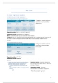
The documents are fully written in English. I made 2 separate documents, one summary for Prof Cools and one for prof Cleeren. This contains all the relevant information that is needed for the exam in January. - Also have a look at my profile for other summaries.
1. Linear regression analysis
1.1 When to use a linear regression?
Linear regression versus logistic regression?
* Categorical variables need to be
converted to dummy variables
(binary: 1/0)!
Dependent variable: Metric or nominal (in logistics)
Independent variable: always Metric or Categorical
Metric: countable variable (you can count with these numbers).
Categorical: male and female, all kinds of values are possible, isn’t a number (you can’t count with it).
You assign a number to the group but the number doesn’t mean anything, random choice of
numbers.
Linear regression versus ANOVA?
* Categorical variables need to be
converted to dummy variables
(binary: 1/0)!
Dependent variable: both Metric
Independent variable: different
Exercise
Dependent variable: “a person´s decision to
buy a private (store) label” ≠ Metric = Nominal
(2 groups → binary)
Independent variable: “consumer
characteristics” ≠ not metric = categorical
→ Test: Binary logistic regression
1
, Dependent variable: “a person´s attitude
towards buying private (store) label” = Likert
scale → considered a Metric variable.
Independent variable: “consumer
characteristics” ≠ not metric = categorical
Independent variable: “consumer
characteristics” ≠ not metric = categorical
→ Multinomial logistic regression
1.2 Creating dummy variables
• Transform categorical independent variables into dummy (1/0) variables (aka indicator
variables) in a linear (and logistic) regression
• Dummy variable trap!
o = if you would include as many dummies as response categories → you create perfect
multicollinearity, you can perfectly predict values of last category based on values of
other categories. If male = 1 → female will be 0.
o # dummies = # response categories – 1
▪ You should include 1 dummy less than the number of response categories.
HOW: Tabulate X, generate(X)
Example linear regression
2
, Control variable = which we know will influence
dependent variable/results, but we are not really
interested in their effect (there will not be a
hypothesis on this). If we do not include them →
omitted variable bias. They will be treated as
independent variables.
Subscript (i) = level of observation !
1.3 Linear regression in Stata
HOW: Regress
1.3.1 Model diagnostics – Steps
• Step 1: Check assumptions (if necessary, apply corrections)
o Assumption 1: Causality.
o Assumption 2: Were all relevant variables included?
o Assumption 3: Metric dependent variable.
o Assumption 4: Linear relationship between dependent and independent variables.
o Assumption 5: Additive relationship between dependent and independent variables.
o Assumption 6: Residuals need to be independent, normally distributed, homoscedastic,
without autocorrelation.
o Assumption 7: Enough observations
o Assumption 8: No multicollinearity
o Assumption 9: No extreme values
• Step 2: Check ‘meaningfulness’ of model (model fit); H0: R² = 0
• Step 3: Interpret the coefficients of each independent variable; H0: bi = 0
Step 1: check assumptions
ASSUMPTION 1: CAUSALITY
• Independent variables (RHS) should be causing the dependent variable.
ASSUMPTION 2: ALL RELEVANT VARIABLES
• No extreme clusters & No striking patterns
HOW: residuals versus fitted (rvf) plot - Predicted variables against residuals
ASSUMPTION 6: NORMAL DISTRIBUTION OF RESIDUALS
HOW visually: Histogram of residuals – should be normally distributed
PP-plot (probability-plot) – should be normally distributed
HOW statistically: Shapiro’s Wilk normality test – H0: residuals normally distributed
! You don’t want to reject H0, residuals will then be normally distributed.
• If violated: check why the standard errors are not normally distributed:
o Problem in model -> fix it!
o Dependent variable not normally distributed -> transformation of dependent variable
(logarithm, square, root)
• Important: if you use a transformation, it has implications for the interpretation of the results !!
(interpret in function of transformed variable).
• If the sample size is large enough → violation of normal distribution usually not a problem
3
Les avantages d'acheter des résumés chez Stuvia:
Qualité garantie par les avis des clients
Les clients de Stuvia ont évalués plus de 700 000 résumés. C'est comme ça que vous savez que vous achetez les meilleurs documents.
L’achat facile et rapide
Vous pouvez payer rapidement avec iDeal, carte de crédit ou Stuvia-crédit pour les résumés. Il n'y a pas d'adhésion nécessaire.
Focus sur l’essentiel
Vos camarades écrivent eux-mêmes les notes d’étude, c’est pourquoi les documents sont toujours fiables et à jour. Cela garantit que vous arrivez rapidement au coeur du matériel.
Foire aux questions
Qu'est-ce que j'obtiens en achetant ce document ?
Vous obtenez un PDF, disponible immédiatement après votre achat. Le document acheté est accessible à tout moment, n'importe où et indéfiniment via votre profil.
Garantie de remboursement : comment ça marche ?
Notre garantie de satisfaction garantit que vous trouverez toujours un document d'étude qui vous convient. Vous remplissez un formulaire et notre équipe du service client s'occupe du reste.
Auprès de qui est-ce que j'achète ce résumé ?
Stuvia est une place de marché. Alors, vous n'achetez donc pas ce document chez nous, mais auprès du vendeur hwstudent2. Stuvia facilite les paiements au vendeur.
Est-ce que j'aurai un abonnement?
Non, vous n'achetez ce résumé que pour €8,99. Vous n'êtes lié à rien après votre achat.