Biot–Savart law
In physics, specifically electromagnetism, the Biot–Savart law (/ˈbiː oʊ sə
ˈvɑː r/ or /ˈbjoʊ səˈvɑː r/) is an equation describing the magnetic field generated
[1]
by a constant electric current. It relates the magnetic field to the magnitude,
direction, length, and proximity of the electric current. The Biot–Savart law is
fundamental to magnetostatics, playing a role similar to that of Coulomb's
law in electrostatics. When magnetostatics does not apply, the Biot–Savart law
should be replaced by Jefimenko's equations. The law is valid in
the magnetostatic approximation, and consistent with both Ampère's circuital
law and Gauss's law for magnetism. It is named after Jean-Baptiste
[2]
Biot and Félix Savart, who discovered this relationship in 1820.
Equation[edit]
Electric currents (along a closed curve/wire)[edit]
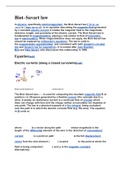
Shown are the directions of , , and the value of
The Biot–Savart law is used for computing the resultant magnetic field B at
[3]: Sec 5-2-1
position r in 3D-space generated by a flexible current I (for example due to a
wire). A steady (or stationary) current is a continual flow of charges which
does not change with time and the charge neither accumulates nor depletes at
any point. The law is a physical example of a line integral, being evaluated
over the path C in which the electric currents flow (e.g. the wire). The equation
in SI units is [4]
where is a vector along the path whose magnitude is the
length of the differential element of the wire in the direction of conventional
current. is a point on path . is the full displacement
vector from the wire element ( ) at point to the point at which the
field is being computed ( ), and μ is the magnetic constant.
0
Alternatively:
, where is the unit vector of . The symbols in boldface
denote vector quantities.
The integral is usually around a closed curve, since stationary electric
currents can only flow around closed paths when they are bounded. However,
the law also applies to infinitely long wires (this concept was used in the
definition of the SI unit of electric current—the Ampere—until 20 May 2019).
To apply the equation, the point in space where the magnetic field is to be
calculated is arbitrarily chosen ( ). Holding that point fixed, the line
integral over the path of the electric current is calculated to find the total
magnetic field at that point. The application of this law implicitly relies on
the superposition principle for magnetic fields, i.e. the fact that the magnetic
field is a vector sum of the field created by each infinitesimal section of the
wire individually.
[5]
An example used in the Helmholtz coil, solenoids and the Magsail spacecraft
propulsion design is the magnetic field at a distance along the center-
line (cl) chosen as the x axis of a loop of radius carrying a current
as follows:
where is the unit vector of from a 1979 physics textbook [3]: Sec 5-2, Eqn
and a website with an on-line calculator. Calculation of the off center-line
(25) [6]
axis magnetic field requires more complex mathematics involving elliptic
integrals that require numerical solution using commercial mathematical tools
or approximations, code, with further details of the derivation given in.
[7] [8] [9]
There is also a 2D version of the Biot–Savart equation, used when the sources
are invariant in one direction. In general, the current need not flow only in a
plane normal to the invariant direction and it is given by [dubious – discuss]
(current
density). The resulting formula is:
Electric current density (throughout conductor volume)[edit]
Les avantages d'acheter des résumés chez Stuvia:
Qualité garantie par les avis des clients
Les clients de Stuvia ont évalués plus de 700 000 résumés. C'est comme ça que vous savez que vous achetez les meilleurs documents.
L’achat facile et rapide
Vous pouvez payer rapidement avec iDeal, carte de crédit ou Stuvia-crédit pour les résumés. Il n'y a pas d'adhésion nécessaire.
Focus sur l’essentiel
Vos camarades écrivent eux-mêmes les notes d’étude, c’est pourquoi les documents sont toujours fiables et à jour. Cela garantit que vous arrivez rapidement au coeur du matériel.
Foire aux questions
Qu'est-ce que j'obtiens en achetant ce document ?
Vous obtenez un PDF, disponible immédiatement après votre achat. Le document acheté est accessible à tout moment, n'importe où et indéfiniment via votre profil.
Garantie de remboursement : comment ça marche ?
Notre garantie de satisfaction garantit que vous trouverez toujours un document d'étude qui vous convient. Vous remplissez un formulaire et notre équipe du service client s'occupe du reste.
Auprès de qui est-ce que j'achète ce résumé ?
Stuvia est une place de marché. Alors, vous n'achetez donc pas ce document chez nous, mais auprès du vendeur anjithaanju. Stuvia facilite les paiements au vendeur.
Est-ce que j'aurai un abonnement?
Non, vous n'achetez ce résumé que pour 4,33 €. Vous n'êtes lié à rien après votre achat.