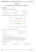
Inventory management subject to
deterministic demand
Inventory management
• Focus on two questions:
o When should an order be placed?
o How much should be ordered?
1 BASIC EOQ MODEL
Relevant costs
• Holding cost
o = carrying cost or inventory cost
o costs proportional to the quantity of inventory held
o cost of keeping €1 in inventory for 1 year
o h = Ic
with item cost c and annual interest rate I
o Includes
▪ Physical cost of space
• Rent/investment, heat, light, equipment
▪ Taxes and insurance
▪ Breakage, spoilage and deterioration
▪ Opportunity C-cost of alternative investment (WACC)
• Order cost
o Cost of placing an order from a supplier
o K
o Includes:
▪ Administration and communication costs
▪ Receiving and quality inspection costs
▪ Fixed transportation costs
Sawtooth pattern:
Q = size of
the order
T = cycle length
1
Operations Management 2019-2020 Casier Tessa
,Minimizing total (annual) costs
• Average annual cost = annual order cost + annual purchase cost + annual holding cost
• EOQ = Q to minimize the average annual cost, G(Q)
𝐾 + 𝑐𝑄 ℎ𝑄
𝐺(𝑄) = + 𝑄
𝑇 2 𝑇 =
𝐾𝜆 ℎ𝑄 𝜆
𝐺(𝑄) = + 𝜆𝑐 +
𝑄 2
with λ the average demand rate
𝐾𝜆 ℎ
𝐺 ′ (𝑄) = − 2 + = 0
𝑄 2
• Economic order quantity (EOQ)
2𝐾𝜆
𝑄∗= √
ℎ
𝜆
This also determines the optimal number of orders per year 𝑄 and the optimal reorder
𝑄
interval 𝑇 ∗= 𝜆 .
• Costs
𝑄
o Average annual holding cost = ℎ 2
𝜆
o Average annual order cost = 𝐾 𝑄
o Average annual purchase cost = 𝜆𝑐
Economic Order Quantity model: trade-off between fixed order cost and holding costs
Assumptions
• Demand rate is deterministic and constant at λ units per unit time
• Shortages are not allowed
• Orders are received instantaneously
• Cost structure:
o Fixed order cost K
o Proportional purchase costs c
o Holding cost at h per unit held per time unit
Remarks:
• Q* is the order quantity for which annual order costs equal annual holding costs
• c does not appear explicitly in the expression for Q*, but c does affect the value of Q*
indirectly because h = Ic
• Even though the EOQ minimizes the yearly holding and setup costs, it could be infeasible,
e.g., space constraint, budget constraint
Robustness of the solution – sensitivity
• Total costs are relatively stable around Q*
• Often better to order a more convenient lot size (or with a more convenient reorder interval)
close to Q*, than the precise Q*
2
Operations Management 2019-2020 Casier Tessa
, • A greater penalty cost if you order too little than too much
𝐾𝜆 ℎ𝑄 2𝐾𝜆
𝐺(𝑄) = 𝑄
+ 2
and 𝑄 ∗= √ ℎ
𝐾𝜆
ℎ 2𝐾𝜆
𝐺∗ = + √
√2𝐾𝜆/ℎ 2 ℎ
𝐾𝜆ℎ
= 2√
2
= √2𝐾𝜆ℎ
𝐺(𝑄) 𝐾𝜆/𝑄 + ℎ𝑄/2
=
𝐺∗ √2𝐾𝜆ℎ
1 2𝐾𝜆 𝑄 ℎ
= √ + √
2𝑄 ℎ 2 2𝐾𝜆
𝑄∗ 𝑄
= +
2𝑄 2𝑄 ∗
1 𝑄∗ 𝑄
= [ + ]
2 𝑄 𝑄∗
The purchase cost λc is neglected because it is not influenced by Q
Inclusion of order lead time ≤ T
• ↔ Basic EOQ assumption: orders are received instantaneously
• Constant order lead time τ ≤ T
• Reorder point, R = level of on-hand inventory at the instant an order should be placed
(R = λτ)
3
Operations Management 2019-2020 Casier Tessa
, 2 EOQ WITH FINITE PRODUCTION RATE: EPQ
Motivation for holding inventories
• Basic EOQ:
o Fixed ordering cost → Economies of scale
CYCLE INVENTORY
• EPQ (Economic Production Quantity)
o Suppose that items are produced internally at a rate P (> λ, the consumption rate)
o There is a fixed setup time/cost per batch → Economies of scale
• Setup (or changeover) cost
o Planning the order
o Lost time (and capacity) due to changeover
o Initial (warm-up) losses after setup
𝐵𝑎𝑡𝑐ℎ 𝑠𝑖𝑧𝑒
𝐶𝑎𝑝𝑎𝑐𝑖𝑡𝑦 𝑔𝑖𝑣𝑒𝑛 𝑏𝑎𝑡𝑐ℎ 𝑠𝑖𝑧𝑒 =
𝑆𝑒𝑡𝑢𝑝 𝑡𝑖𝑚𝑒 + 𝐵𝑎𝑡𝑐ℎ 𝑠𝑖𝑧𝑒 × 𝑇𝑖𝑚𝑒 𝑝𝑒𝑟 𝑢𝑛𝑖𝑡
EOQ with finite production rate
𝑄 = 𝑃 × 𝑇1
𝐻 = (𝑃 − 𝜆) × 𝑇1
𝑄
𝐻 = (𝑃 − 𝜆) ×
𝑃
𝜆
𝐻 = 𝑄 × (1 − )
𝑃
𝐾 ℎ𝐻
𝐺(𝑄) = + + 𝜆𝑐
𝑇 2
𝐾𝑄 ℎ𝑄 𝜆
𝐺(𝑄) = + (1 − ) + 𝜆𝑐
𝜆 2 𝑃
• The optimal production quantity to minimize average annual holding and set up costs has the
same form as the EOQ
• Minimizing total (annual) costs
𝐾𝑄 ℎ𝑄 𝜆
𝐺(𝑄) = + (1 − ) + 𝜆𝑐
𝜆 2 𝑃
1−𝜆
with: h’ = ℎ
𝑃
𝐾𝜆 ℎ′
𝐺′(𝑄) = − 2 + = 0
𝑄 2
• Economic production quantity (EOQ)
2𝐾𝜆
𝑄 ∗= √
ℎ′
4
Operations Management 2019-2020 Casier Tessa