Summary

Summary Linear Algebra Notes

7 views 0 purchase

Course
Algebra 1: Linear Algebra (MATH240)

Institution
Simon Fraser University (SFU )

These notes cover chapters 1, 2, 3, 4, the theory bases subsections in chapters 5 and 6, and then the first subsection in chapter 7. I have noted theorems from the book and elaborated on my understanding of the subject in a clear and concise manner. This is all rigorous theory, with little applicat...

[Show more]

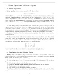
Preview 3 out of 25 pages

View example

Summarized whole book? No
Which chapters are summarized? 1-7
Uploaded on January 2, 2022
Number of pages 25
Written in 2021/2022
Type Summary

linear algebra
matrix
augmented matrix
coefficient matrix
algebra
echelon form
linear independence
linear dependence
vector
eigenvalue
linear transformation
subspace
vector space
subspace test
rank
co

CA$17.39

Added

Add to cart Add to wishlist

100% satisfaction guarantee
Immediately available after payment
Both online and in PDF
No strings attached

1 Linear Equations in Linear Algebra
1.1 Linear Equations
A linear equation, where x1 , x2 , ..., xn and n ∈ N, takes the form
a1 x1 + · · · + an xn = b, (1)
with coe
cients a1 , ..., an ∈ C , R. A linear system is two or more linear equations with the same
variables. A solution set of a linear system is the set of all solutions, S = {sn ∈ R | s1 , ..., sn },
which is equivalent to another if they both have set S . Consistent with either one or in
nitely
many solutions, and inconsistent with no solutions. We can have either a Coe
cient matrix,
using coe
cients of x1 , x2 , ..., xn , or an augmented matrix, adding the RHS constants. An m
× n matrix has m rows and n columns.

A basic solving strategy, using elementary row operations, is to replace one system with an
equivalent system that is easier to solve : we replace one equation, R, by the sum of itself and a
multiple of another equation, L, so R∗ = R + nL, interchange equations, and multiply all terms
in an equation by a nonzero constant (scaling). Two matrices are row equivalent if a sequence
of elementary row equations transforms one matrix to another. Row operations are reversible.
If augmented matrices of two linear systems are row equivalent, then the two systems have the
same solution set.

Fundamental Questions: Is the system consistent, does at least one solution exist ? If a solution
exists, is it unique ? In triangular form, say we know one solution value, we can use a variable
to solve another equation and so on, until we have a complete solution. If all solution values are
determined by another value, then it is unique. If a matrix looks like
 
2 −3 2 1
0 1 −4 8 
0 0 0 15

then we note, by the
nal row, the system is inconsistent in triangular form.

1.2 Row Reduction and Echelon Forms
A leading entry is the leftmost entry in a nonzero row, where a nonzero row or column in a
matrix means a row or column with at least one nonzero entry. A rectangular matrix is in echelon
form if it has the following three properties:
1. All nonzero rows are above any rows of all zeros.
2. Each leading entry of a row is in a column to the right of the leading entry of the row above
it.
3. All entries in a column below a leading entry are zeros.
A matrix is in reduced echelon form if the following conditions are also satis
ed:
4. The leading entry in each nonzero row is 1.
5. Each leading 1 is the only nonzero entry in its column
An echelon matrix takes echelon form, reduced echelon matrix takes reduced echelon
form.

1

,Theorem 1.1 (Uniqueness of the Reduced Echelon Form) Each matrix is row equivalent
to one and only one reduced echelon matrix.
If matrix A is row equivalent to an echelon matrix U , we call U an echelon form of A; and
the respective case where U is the reduced echelon form of A. The leading entries are always
in the same positions in any echelon form obtained from a given matrix.
A pivot position in a matrix A is a position in A that corresponds to a leading 1 in the
reduced echelon form of A. A pivot column is a column of A containing a pivot position. A
pivot, de
ned by {p ∈ R | p ̸= 0}, is used as needed to create zeroes via row operations.
The forward phase of the row reduction algorithm is to locate the top left pivot column and
select a nonzero entry, and use replacement operations to create zeros in the positions below the
pivot. Then repeat the process, omitting the row with the pivot position, until there are no more
nonzero rows to modify. The backward phase begins with the rightmost pivot, moving upward
and to the left, creating zeros above that pivot, and then scaling the pivot to 1.

A basic variable lies in a pivot column, and a free variable can be represented as a basic
variable.
Theorem 1.2 (Existence and Uniqueness Theorem) A linear system is consistent i the
rightmost column of the augmented matrix is not a pivot column. That is, i an echelon form
of the augmented matrix has no row of form
b

0 ... 0

If a linear system is consistent, then the solution set contains either (i) a unique solution, no free
variables, or (ii) in
nitely many solutions with at least one free variable.
This theorem answers the questions present in 1.1, as given by the theorem name.

Using Row Reduction to Solve a Linear System
1. Write the augmented matrix of the system.
2. Use row reduction algorithm to obtain an equivalent augmented matrix in echelon form.
3. Obtain reduced echelon form.
4. Write in terms of a system of equations
5. Express all nonzero equations so its one basic variable is in terms of any free variables.
A
op is one arithmetic operation.

1.3 Vector Equations
A column vector, v, is an ordered set of n entries, written
 
v1
 ...  ,
vn

for now v ∈ Rn . (vector
elds) The zero vector, 0, will be determined by context.

Algebraic Properties of Rn

2

, Commutativity - u + v = v + u
Associativity - (u + v) + w = u + (v + w)
Additive Identity - u + 0 = 0 + u = u
Additive Inverse - u + (−u) = −u + u = 0
Distribution of Vector Sums - c(u + v) = cv + cu
Distribution of Scalar Sums - u(c + d) = uc + ud
Associativity of Scalar Multiplication - c(du) = (cd)u
Multiplicative Identity - 1u = u
Parallelogram Rule of Addition
If v and u in R2 are points on a plane, then v + u corresponds to the fourth vertex of the
parallelogram with vertices also at O, v, and u.
Given vectors v1 , v2 , ..., vp in Rn and given corresponding scalars, the vector y de
ned by
y = c1 v1 + ... + cp vp
is a linear combination of the vectors with corresponding weights.
A vector equation,
x1 a1 + x2 a2 + ... + xn an = b,
has the same solution set as the linear system whose augmented matrix is
a1 a2 ... an b ,

where b can be generated by a linear combination of a1 , ... , an i there exists a solution corre-
sponding to the augmented matrix.
Key Idea of Linear Algebra - Study the set of all vectors that can be generated/written as
a linear combination of a
xed set of vectors.
De
nition 1 If v1 , ... , vp are in Rn , then the set of all linear combinations of those vectors is
denoted by
Span{v1 , ... , vp }
and is called the subset of Rn spanned by v1 , ... , vp : it is the collection of all vectors that can
be written in linear combination form with scalars c1 , ... , cp .
Asking if b is in Span{v1 , ... , vp } amounts to asking whether the vector equation x1 v1 +
x2 v2 + ... + xn vp = b has a solution, or, equivalently, asking whether the system with augmented
matrix v1 v2 ... vp b has a solution.

1.4 The Matrix Equation (Ax = b)
De
nition 2 If A is an m × n matrix, with columns a1 , ... , an and if x is in Rn , then the product
of A and x, denoted by Ax, is the linear combination of A using the corresponding entries in x as
weights; that is,  
x1
 x2 
Ax = a1 a2 ... an 

 ...  ,


xn
which is only de
ned when the number of columns in A equals the number of entries in x.

3

The benefits of buying summaries with Stuvia:

Guaranteed quality through customer reviews

Stuvia customers have reviewed more than 700,000 summaries. This how you know that you are buying the best documents.

Quick and easy check-out

You can quickly pay through credit card or Stuvia-credit for the summaries. There is no membership needed.

Focus on what matters

Your fellow students write the study notes themselves, which is why the documents are always reliable and up-to-date. This ensures you quickly get to the core!

Frequently asked questions

What do I get when I buy this document?

You get a PDF, available immediately after your purchase. The purchased document is accessible anytime, anywhere and indefinitely through your profile.

Satisfaction guarantee: how does it work?

Our satisfaction guarantee ensures that you always find a study document that suits you well. You fill out a form, and our customer service team takes care of the rest.

Who am I buying these notes from?

Stuvia is a marketplace, so you are not buying this document from us, but from seller TheQuantitativeNoteMan. Stuvia facilitates payment to the seller.

Will I be stuck with a subscription?

No, you only buy these notes for CA$17.39. You're not tied to anything after your purchase.

Can Stuvia be trusted?

4.6 stars on Google & Trustpilot (+1000 reviews)

76449 documents were sold in the last 30 days

Founded in 2010, the go-to place to buy study notes for 14 years now

Start selling

Summary

Summary Linear Algebra Notes

Document information

Subjects

Connected book

Written for

Seller

Content preview