100% satisfaction guarantee Immediately available after payment Both online and in PDF No strings attached
logo-home
Summaries of all lecture notes in APM346, you will be good to go if you are able to understand everything shown in the notes CA$11.92
Add to cart

Class notes

Summaries of all lecture notes in APM346, you will be good to go if you are able to understand everything shown in the notes

 0 purchase

Summaries of all lecture notes in APM346, you will be good to go if you are able to understand everything shown in the notes

Preview 3 out of 16  pages

  • December 12, 2022
  • 16
  • 2019/2020
  • Class notes
  • Unknown
  • All classes
All documents for this subject (11)
avatar-seller
9kfhgia89h1
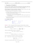
July 21, 2020 APM346 – Week 9 Justin Ko


1 Separation of Variables I
Our goal is to develop a technique to solve IBVPs on the finite interval. This method is called separa-
tion of variables and it reduces the IBVP into a system of ODEs. This approach will give us a series
representation of the solution, that will converge to the true solution of the IBVP.

We first explain how one would do separation of variables in the easiest case when we have a ho-
mogeneous PDE with homogeneous boundary conditions.

1. Assume the solution u(x, t) is of the form u(x, t) = X(x)T (t).
2. Use linearity to write the general solution as an infinite linear combination of general solutions
that satisfy the PDE and boundary conditions:
(a) Spatial Problem: Solve the spatial eigenvalue problem.
(b) Time Problem: Solve the system of homogeneous time ODEs using the eigenvalues from
the spatial problem.
3. Use the initial conditions to solve for the particular solution from the general solution using the
appropriate Fourier coefficients.

1.1 Example Problems
Problem 1.1. (?) Solve


utt − c2 uxx = 0 0 < x < π, t > 0

u|
t=0 = 0 0<x<π


ut |t=0 = x 0<x<π
ux |x=0 = ux |x=π = 0 t > 0.


Solution 1.1. This is a homogeneous PDE with homogeneous Neumann boundary conditions.

Step 1 — Separation of Variables: We look for a separated solution u(x, t) = X(x)T (t) to our IBVP.
Plugging this into the BVP implies

T 00 (t) X 00 (x)
T 00 (t)X(x) − c2 T (t)X 00 (x) = 0 =⇒ 2
= = −λ.
c T (t) X(x)

This gives the following ODEs (see Remark 1 and Remark 2)

X 00 (x) + λX(x) = 0 and T 00 (t) + c2 λT (t) = 0,

with boundary conditions

T (t)X 0 (0) = T (t)X 0 (π) = 0 =⇒ X 0 (0) = X 0 (π) = 0

since we can assume T (t) 6≡ 0 otherwise we will have a trivial solution.

Step 2 — Spatial Problem: We begin by solving the eigenvalue problem
(
−X 00 = λX 0<x<π
X 0 (0) = X 0 (π) = 0.

The solution to the eigenvalue problem (Week 7 Lecture Summary 1.1.2) is


Page 1 of 16

,July 21, 2020 APM346 – Week 9 Justin Ko


Eigenvalues: λn = n2 for n = 0, 1, 2, . . .
Eigenfunctions: Xn = cos(nx) and X0 = 1.
Step 3 — Time Problem: When n = 0, the time problem is
T000 (t) = 0
which has solution
T0 (t) = A0 + B0 t.
The time problem related to the eigenvalues λn for n ≥ 1 is
Tn00 (t) + c2 n2 Tn (t) = 0 for n = 1, 2, . . .
which has solution
Tn (t) = An cos(cnt) + Bn sin(cnt).
Step 4 — General Solution: By the principle of superposition, the general form of our solution is

X ∞ 
X 
u(x, t) = Tn (t)Xn (x) = A0 + B0 t + An cos(cnt) + Bn sin(cnt) cos(nx).
n=1 n=1

Step 5 — Particular Solution: We now use the initial conditions to recover the particular solution by
solving for the constants An and Bn . The initial conditions imply

X
u(x, 0) = 0 =⇒ A0 + An cos(nx) = 0
n=1

and

X
ut (x, 0) = x =⇒ B0 + Bn cn cos(nx) = x.
n=1
Clearly the first initial condition implies that An = 0 for all n ≥ 0. To find the Bn coefficients, we
decompose x into its Fourier cosine series (or equivalently, decomposing |x| into its full Fourier series
on [−π, π])

π X 2((−1)n − 1)
x= + cos(nx)
2 n=1 πn2
and equate coefficients to conclude
π 2((−1)n − 1) 2((−1)n − 1)
B0 = , Bn cn = 2
=⇒ Bn = .
2 πn cπn3
Therefore, our particular solution is

X
u(x, t) = B0 t + Bn sin(cnt) cos(nx)
n=1

π 2((−1)n −1)
where B0 = 2 and Bn = cπn3 .
Remark 1. In general, if
f (x) = g(t)
for all x and t, then there must exist a C such that f (x) = g(t) = C. To see why, we can take the
partial derivatives to conclude that
∂x f (x) = ∂x g(t) = 0 and ∂t g(t) = ∂t f (x) = 0,
so both f and g must be constant by the mean value theorem. Since f (x) = g(t), this implies the
constant must be the same.


Page 2 of 16

, July 21, 2020 APM346 – Week 9 Justin Ko


Remark 2. We will explain how one can rigorously justify the fact that

T 00 (t)X(x) − c2 T (t)X 00 (x) = 0 =⇒ X 00 (x) + λX(x) = 0 and T 00 (t) + c2 λT (t) = 0

for some λ. Since we are interested in non-trivial solutions, there exists a x0 such that X(x0 ) 6= 0.
This implies that
X 00 (x0 )
T 00 (t)X(x0 ) − c2 T (t)X 00 (x0 ) = 0 =⇒ T 00 (t) − c2 T (t) = 0 =⇒ T 00 (t) + c2 λT (t) = 0
X(x0 )
00
where λ1 := − XX(x (x0 )
0)
. Similarly, for a non-trivial solution to exist, there must be a t0 such that
T (t0 ) 6= 0, which will imply
T 00 (t0 )
T 00 (t0 )X(x) − c2 T (t0 )X 00 (x) = 0 =⇒ X 00 (x) − X(x) = 0 =⇒ X 00 (x) + λ2 X(x) = 0
c2 T (t0 )
00
where λ2 := − cT2 T(t(t00)) . To see why λ1 = λ2 , we can evaluate our original equation at (x0 , t0 ) and use
the fact −λ1 X(x0 ) = X 00 (x0 ) and −c2 λ2 T (t0 ) = T 00 (t0 ) to see that

T 00 (t0 )X(x0 ) − c2 T (t0 )X 00 (x0 ) = 0 =⇒ c2 T (t0 )X(x0 )(λ1 − λ2 ) = 0 =⇒ λ1 = λ2

since c2 T (t0 )X(x0 ) 6= 0. A similar procedure can be done to formally justify “dividing by zero” in all
separation of variables problems.

Problem 1.2. (??) Solve


 utt − c2 uxx = 0 0 < x < L, t > 0

u|
t=0 = g(x) 0<x<L


 ut |t=0 = h(x) 0<x<L
ux |x=0 = u|x=L = 0 t > 0.


Solution 1.2. This is a homogeneous problem with homogeneous boundary conditions.

Step 1 — Separation of Variables: We look for a separated solution u(x, t) = X(x)T (t) to our IBVP.
Plugging this into the BVP implies
T 00 (t) X 00 (x)
T 00 (t)X(x) − kT (t)X 00 (x) = 0 =⇒ 2
= = −λ.
c T (t) X(x)
This gives the following ODEs

X 00 (x) + λX(x) = 0 and T 00 (t) + c2 λT (t) = 0,

with boundary conditions

T (t)X 0 (0) = 0 = T (t)X(L) =⇒ X 0 (0) = X(L) = 0

since we can assume T (t) 6≡ 0 otherwise we will have a trivial solution.

Step 2 — Spatial Problem: We begin by solving the eigenvalue problem
(
−X 00 = λX 0<x<L
0
X (0) = X(L) = 0.

The solution to the eigenvalue problem (Week 7 Lecture Summary 1.1.5) is


Page 3 of 16

The benefits of buying summaries with Stuvia:

Guaranteed quality through customer reviews

Guaranteed quality through customer reviews

Stuvia customers have reviewed more than 700,000 summaries. This how you know that you are buying the best documents.

Quick and easy check-out

Quick and easy check-out

You can quickly pay through credit card or Stuvia-credit for the summaries. There is no membership needed.

Focus on what matters

Focus on what matters

Your fellow students write the study notes themselves, which is why the documents are always reliable and up-to-date. This ensures you quickly get to the core!

Frequently asked questions

What do I get when I buy this document?

You get a PDF, available immediately after your purchase. The purchased document is accessible anytime, anywhere and indefinitely through your profile.

Satisfaction guarantee: how does it work?

Our satisfaction guarantee ensures that you always find a study document that suits you well. You fill out a form, and our customer service team takes care of the rest.

Who am I buying these notes from?

Stuvia is a marketplace, so you are not buying this document from us, but from seller 9kfhgia89h1. Stuvia facilitates payment to the seller.

Will I be stuck with a subscription?

No, you only buy these notes for CA$11.92. You're not tied to anything after your purchase.

Can Stuvia be trusted?

4.6 stars on Google & Trustpilot (+1000 reviews)

68736 documents were sold in the last 30 days

Founded in 2010, the go-to place to buy study notes for 15 years now

Start selling
CA$11.92
  • (0)
Add to cart
Added