100% satisfaction guarantee Immediately available after payment Both online and in PDF No strings attached
logo-home
Complete Solution Manual Introductory Econometrics A Modern Approach 6th Edition Wooldridge (Chapter 1-19) CA$42.65   Add to cart

Exam (elaborations)

Complete Solution Manual Introductory Econometrics A Modern Approach 6th Edition Wooldridge (Chapter 1-19)

 242 views  4 purchases
  • Course
  • Econometrics
  • Institution
  • Econometrics
  • Book

Introductory Econometrics A Modern Approach 6th Edition Wooldridge Solutions Manual Complete Solution Manual Introductory Econometrics A Modern Approach 6th Edition Wooldridge (Chapter 1-19) PDF File All Pages All Chapters Grade A+

Preview 4 out of 471  pages

  • June 21, 2023
  • 471
  • 2022/2023
  • Exam (elaborations)
  • Questions & answers
  • Econometrics
  • Econometrics
avatar-seller
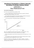
Introductory Econometrics A Modern Approach 6th Edition Wooldridge Solutions Manual APPENDIX A Basic Mathematical Tools SOLUTIONS TO PROBLEMS A.1 (i) The average monthly housing expenditure is $566. (ii) The two middle numbers are 480 and 530; when these are averaged, we obtain the median monthly housing expenditure as 505, or $505. (iii) If monthly housing expenditures are measured in hundreds of dollars, the average and median monthly housing expenditures are 5.66 and 5.05, respectively. (iv) The average increases to $586 while the median is unchanged ($505). A.2 (i) This is just a standard linear equation with intercept equal to 3 and slope equal to .2. The intercept is the number of classes missed by a student who lives on campus. (ii) The average number of classes missed for someone who lives five miles away is 3 + .2(5) = 4 classes. (iii) The difference in the average number of classes missed for someone who lives 10 miles away and someone who lives 20 miles away is 10(.2) = 2 classes. A.3 If price = 15 and income = 200, quantity = 120 – 9.8(15) + .03(200) = –21, which is nonsense. This shows that linear demand functions generally cannot describe demand over a wide range of prices and income. A.4 (i) The percentage point change is 5.6 – 6.4 = –.8, or an eight -tenths of a percentage point decrease in the unemployment rate. (ii) The percentage change in the unemployment rate is 100[(5.6 – 6.4)/6.4] = –12.5%. A.5 The majority shareholder is referring to the percentage point increase in the stock return, while the CEO is referring to the change relative to the initial return of 15%. To be precise, the shareho lder should specifically refer to a three percentage point increase. A.6 (i) The exact percentage by which Person B’s salary exceeds Person A’s is 100[42,000 – 35,000)/35,000] = 20%. (ii) The approximate proportionate change is log(42,000) – log(35,000)  .182, so the approximate percentage change is 18.2%. [Note: log() denotes the natural log.] A.7 (i) When exper = 0, log(salary ) = 10.6; therefore, salary = exp(10.6)  $40,134.84. When exper = 5, salary = exp[10.6 + .027(5)]  $45,935.80. (ii) The approximate proportionate increase in salary when exper increases by five years is .027(5) = .135, so the approximate percentage change is 13.5%. (iii) 100[(45,935.80 – 40,134.84)/40,134.84)  14.5%, so the exact percentage increase is about one percentage point higher. A.8 From the given equation, grthemp = –.78(salestax ). Since both variables are in proportion form, we can multiply the equation through by 100 to turn each variable into percentage form. This leaves the slope as –.78. So, a one percentage point increase in the sales tax rate (say, from 4% to 5%) reduces employment growth by –.78 percentage points. A.9 (i) The relationship between yield and fertilizer is graphed below. yield 122 121 120 0 50 100 fertilizer (ii) Compared with a linear function, the function yield = 120 + .19 has a diminishing effect, and the slope approaches zero as fertilizer gets large. The initial pound of fertilizer has the largest effect, and each additional pound has an effect smaller than the previous pound. A.10 (i) The value 45.6 is the intercept in the equation, so it literally means that if class = 0, then the score is 45.6. Of course, class = 0 can n ever happen. And values close to zero would rarely if ever occur, except in very small schools. So, by itself, 45.6 is not of much interest. But it must be accounted for to use the equation to obtain score for sensible values of class . (ii) We use calculus to obtain the optimal class size: class*  .082 / [2(.000147)]  278.91 . Rounded to the nearest integer, the optimal class size is 279 students. When we plug this into the equation for score , we get the largest achievable score: score*  45.6 .082(279) .000147(2792 )  57.04 . (iii) The following graph shows the solution rounded to the nearest integer: fertilizer (iv) It is not at all realistic to think that a student’s score is determined only by the size of his or her graduating class. For one thing, that would imply that all students graduating in the same year from the same high school would have the same score. A s tudent’s ability, motivation, classes taken, family background, and many other factors – including some that are totally random, such as not feeling well while taking the test – would come into play. In fact, it is safe to say that, realistically, the size of the graduating class would have a small effect, if any effect at all. Multiple regression analysis allows for many observed factors to affect a variable like score , and it also recognizes that there are unobserved factors that are important and that we can never directly account for. A.11 (i) Let (𝑥1, 𝑦1) and (𝑥2, 𝑦2) be two points on the line 𝑦 = 𝛽0 + 𝛽1𝑥. Using summation operator, 2 2 � 𝑦𝑖𝑖 = 2𝛽0 + 𝛽1 � 𝑥𝑖𝑖 𝑖𝑖=1 2 𝑖𝑖=1 2 2𝛽0 = � 𝑦𝑖𝑖 − 𝛽1 � 𝑥𝑖𝑖 𝑖𝑖=1 𝑖𝑖=1 𝛽0 = (𝑦1 + 𝑦2)/2 − 𝛽1[(𝑥1 + 𝑥2)/2] 𝛽0 = 𝑦 − 𝛽1𝑥 Therefore, (𝑥, 𝑦) is on the line 𝑦 = 𝛽0 + 𝛽1𝑥. 200 279 350 class score 57 52 53 54 55 56

The benefits of buying summaries with Stuvia:

Guaranteed quality through customer reviews

Guaranteed quality through customer reviews

Stuvia customers have reviewed more than 700,000 summaries. This how you know that you are buying the best documents.

Quick and easy check-out

Quick and easy check-out

You can quickly pay through credit card or Stuvia-credit for the summaries. There is no membership needed.

Focus on what matters

Focus on what matters

Your fellow students write the study notes themselves, which is why the documents are always reliable and up-to-date. This ensures you quickly get to the core!

Frequently asked questions

What do I get when I buy this document?

You get a PDF, available immediately after your purchase. The purchased document is accessible anytime, anywhere and indefinitely through your profile.

Satisfaction guarantee: how does it work?

Our satisfaction guarantee ensures that you always find a study document that suits you well. You fill out a form, and our customer service team takes care of the rest.

Who am I buying these notes from?

Stuvia is a marketplace, so you are not buying this document from us, but from seller gradexam. Stuvia facilitates payment to the seller.

Will I be stuck with a subscription?

No, you only buy these notes for CA$42.65. You're not tied to anything after your purchase.

Can Stuvia be trusted?

4.6 stars on Google & Trustpilot (+1000 reviews)

77764 documents were sold in the last 30 days

Founded in 2010, the go-to place to buy study notes for 14 years now

Start selling
CA$42.65  4x  sold
  • (0)
  Add to cart