Op Research Summary Notes
Linear Programming
Target maximisation is described by Z: an objective function
Graphical Method: 2D or 3D, change all ‘subjective to’ lines equal to1 for gradients (if high), make sure
all variables on one side, make sure the inequalities are correct. Min or Max will be along the edge of the
feasible region (shade this region).
Intersection points found by A and b, making an augmented matrix (A|b). Turning A into an REF will
solve for the intersection point.
Table of values looks at the objective function and the value of Z with each variable pairing.
Ex. Kite, Tilted Trapezium, Mootastic (most likely stated but in full notes if needed)
Standard Max Form:
Z = 𝒄𝑻 x
Ax ≤ b
x ≥ 𝟎𝒏
Standard Min to Standard Max: Obj Fun min(Z) = max(-Z), constraints: expression(1) ≥ expression(2)
goes to -expression(1) ≤ -expression(2)
Z = 𝒄𝑻 x
Canonical Form: Ax = b
x ≥ 𝟎𝒏
Canonical to Stan. Max: = goes into 2 inequalities, then placed as constrains
Stan. Max to Canonical: Add non-negative slack variables to change inequalities in equalities such that
x → x’, c → c’, b, A → A’ = (A|I). If ≤ bi, then add si. If ≥ bi, then minus si and leave other x signs.
Geometry of Systems of Linear Inequalities
Convexity: p2 S in 𝑅𝑛 (non-empty) is convex if for all y1, y2 in S, and lambda in [0,1]:
y = lambda y1 + (1-lambda) y2 is in S
p1
convex
p1 p1 non-convex
p1 p2
p2 non-convex p2
Closed convex: includes its boundaries
Prop 2.1: the intersection of any finite collection of convex sets is convex (proof in ps2),
Complex combination: 𝒚 = ∑𝑛𝑖=1 λ𝑖 𝑦𝑖 𝑤ℎ𝑒𝑟𝑒 𝑖 ≥ 0 𝑎𝑛𝑑 ∑𝑛𝑖=1 λ𝑖 = 1
Hyperplane: 𝐻 ≔ {𝒙 ∈ 𝑅 𝑛 : 𝒏𝑻 𝒙 = 𝑑} (a closed, convex set)
Positive half-space: 𝐻+ ≔ {𝒙 ∈ 𝑅 𝑛 : 𝒏𝑻 𝒙 ≥ 𝑑} (a closed, convex set)
Negative half-space: 𝐻− ≔ {𝒙 ∈ 𝑅 𝑛 : 𝒏𝑻 𝒙 ≤ 𝑑} (a closed, convex set)
Polyhedron: intersection of finite number of half-spaces (if bounded: polytope, if closed: closed
convex set)
, Extreme point: x in S, no 2 points v, w in S: x = lambda v + (1-lambda) w
Basis: LI columns of A, any variables in this are a ‘basic variable’
Basic Solution: x ( Ax = b ) with all n-m non-basic variables equal to 0 (if all 𝑥𝑖 non-negative, becomes a
basic feasible solution)
Rank A = # L.I rows or columns (for nxn matrix, if rankA=n then A is invertible)
Degenerate Solutions: basic solns with 1 or more basis variables equal to 0
x is a basic feasible solution for an LP problem ↔ x is an extreme point of 𝐹(𝑐)
Fundamental Theorem: (a) feasible solution → basic feasible solution, (b) optimal feasible solution →
optimal basic feasible solution
optimal basic feasible solution
optimal feasible solution
feasible solution
basic feasible solution
Simplex Method
allows us to explore the basic feasible soln in a fast and systematic way
Ax = b, A = ( B N ) with B invertible: 𝑥𝐵 + 𝐵−1 𝑁𝑥𝑁 = 𝐵−1 𝑏
𝑍 = 𝑐𝐵𝑇 𝐵−1 𝑏 + (𝑐𝑁𝑇 − 𝑐𝐵𝑇 𝐵−1 𝑁) 𝑥𝑁
vector of reduced costs: 𝑟 𝑇 = 𝑐𝑁𝑇 − 𝑐𝐵𝑇 𝐵−1 𝑁
Z can be increased if the vector of reduced costs has at least one strictly positive component (simplex
tries to swap a basic variable with a non-basic variable to increase Z). 𝑍 = 𝑐𝐵𝑇 𝐵−1 𝑁 + ∑𝑛−𝑚
𝑗=1 𝑟𝑗 𝑥𝑗
Motivating example: places Z=0, write out A and b with the addition of slack variables, tableau 1, most
negative, see if to discard s1 or s2 and check feasibility, find inverse using row operations, which basic
variable to discard, find a pivot, repeat until no negatives
𝒓𝒋 𝜽𝒋 Method
1st Guiding Principle: select the non-basic variable corresponding to the largest 𝑟𝑗 𝑥𝑗
• 𝛼 = 𝛽 −1 𝑁
• 𝛽 = 𝛽 −1 𝒃
• only interested in 𝛼𝑖𝑗 > 0
𝛽
2nd Guiding Principle: 𝑋𝑚+𝑗 = 𝑚𝑖𝑛𝑖=1,…,𝑚 {𝛼 𝑖 ∶ 𝛼𝑖𝑗 > 0} = 𝜃𝑗 and 𝑍 = 𝒄𝛽𝑇 𝛽 −1 𝒃 + 𝑟𝑗 𝜃𝑗
𝑖𝑗
𝑟𝑗 𝜃𝑗 method example: make a tableau,
𝛽
𝜃𝑗 first: for x1, min of 𝛼 𝑖 where 𝛼𝑖𝑗 is positive (move along column 𝑥1 , down and skip any negatives), say
𝑖𝑗
which slack variable the minimum corresponds to discarding, repeat for all 𝑥𝑖 ′𝑠
then 𝑟𝑗 𝜃𝑗 : 𝑟𝑗 will look at the value each 𝑥𝑖 holds in Z (before moving all to the other side), times these r’s
by the found minimums, the max of these says which variable to include and which slack variable to
discard. if 2 have the same max value, select highest rj column (if still, then lowest index column)