In this lecture, we will learn about
- Derive the 3-equation model (in the closed economy): IS, PC and MR curves
- Use the 3-equation model to analyse the effects of a temporary demand shock
The 3-equation model
The 3-equation model consists of the following
- IS curve: 𝒚𝒕 = 𝑨 − 𝒂𝒓𝒕−𝟏
- PC (Phillips) curve: 𝝅𝒕 = 𝝅𝒕−𝟏 + 𝜶(𝒚𝒕 − 𝒚𝒆 )
- MR curve: (𝒚𝒕 − 𝒚𝒆 ) = −𝜶𝜷(𝝅𝒕 − 𝝅𝑻 )
The IS curve models the demand side, the PC curve models the supply side and the MR curve models
the behaviour of the policy maker.
The (dynamic) IS curve
It is given by 𝑦𝑡 = 𝐴 − 𝑎𝑟𝑡−1 where 𝑦𝑡 is the output and 𝑎𝑟𝑡−1 is the real interest rate. It captures
the fact that AD responds negatively to the real interest rate with one period lag.
It is in line with empirical evidence, for example, the Bank of England stated in 1999:
“the empirical evidence is that on average it takes up to about one year in this and other industrial
economies for the response to a monetary policy change to have its peak effect on demand and
production”.
The Phillips curve (with adaptive expectations)
The Phillips curve shows how output and inflation move together in the short run. The starting point
of the Phillips curve is the medium run equilibrium which is given by the intersection of wage setting
and price setting (as shown in the diagram below).
We assume nominal rigidities which means that nominal wages and price do not adjust immediately
to fluctuations in AD – prices and wages are sticky. Firms only adjust wages at the start of each
‘wage round’, so wages stay fixed throughout each ‘wage round’, which is typically a year (Barattieri
et al., 2010).
Prices are adjusted right after the change in wages (in line with evidence, e.g. Alvarez et al., 2005).
Thus, an AD shock’s effect are modelled as follows
- AD shock -> output and employment change
- Next wage round -> nominal wages change
- Immediately after the wage round -> prices change
The output gap is defined by 𝑦𝑡 − 𝑦𝑒 (output minus equilibrium level).
,Wage setters change wages to cover the previous period’s inflation and to reflect the output gap
(e.g. due to AD shocks):
𝛥𝑊 𝛥𝑃
( 𝑊 )𝑡 ≈ ( 𝑃 ) + 𝛼(𝑦𝑡 − 𝑦𝑒 ) (wage inflation)
𝑡−1
Price setters set P immediately after this to keep the mark-up fixed:
𝛥𝑃 𝛥𝑊
( 𝑃 )𝑡 = ( 𝑊 )𝑡 (price inflation)
Substituting the wage inflation into the price inflation equations, we get the Phillips curve:
𝛥𝑃 𝛥𝑃
( ) =( ) + 𝛼(𝑦𝑡 − 𝑦𝑒 ) ⇒ 𝜋𝑡 = 𝜋𝑡−1 + 𝛼(𝑦𝑡 − 𝑦𝑒 )
𝑃 𝑡 𝑃 𝑡−1
⇒ current inflation = lagged inflation + output gap
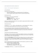
The Phillips curve
We start at the equilibrium level (point A) where we have the equilibrium level of output and
inflation level of 2%. If there is now a positive AD (demand) shock, we have increased employment
(𝑦𝐻 ) and worker’s power in the labour market increases and they ask for higher wages (by 2%). As a
result, wage-setters set higher wages to cover 𝜋𝑡−1 (inflation from the last period) (2%) and the
output gap (2%) (because of less unemployment) (so 4% in total).
Price setters set higher prices to cover higher wage costs and so there is price inflation from 2% to
4%.
Therefore, a positive output gap causes wage and price inflation to rise. At the higher level of output
when inflation is equal to 4%, we get to point B. If we join points A and B, we get the Phillips curve.
Now, price inflation (4%) is 2% higher than expected by wage-setters (2%). In the next wage round,
they will increase wages by an additional 2% to cover the expected inflation erosion of their real
wages. Nominal wages increase by 4% + 2% and so do prices. Price inflation is now 6%. The new PC
curve is given by A’C (above).
,This inflationary pressure in the economy could be resolved in two ways: supply-side or demand-side
policies.
Inflation targeting and the Central Bank
The monetary rule curve
1. Define the central bank’s preferences in terms of deviations from inflation target and equilibrium
output
The central bank’s preferences are given by a loss function (Taylor, 1993):
𝐿 = (𝑦𝑡 − 𝑦𝑒 )2 + 𝛽(𝜋𝑡 − 𝜋 𝑇 )2
The central bank is worse off the further inflation (𝜋𝑡 ) is away from its target level (𝜋 𝑇 ), and the
further output (𝑦𝑡 ) is away from its equilibrium level (𝑦𝑒 ). 𝛽 reflects the relative degree of inflation
aversion of the central bank.
There are two implications of taking the square of these distances
- Levels below the equilibrium are as a bad as levels above the equilibrium
- The more we deviate from the target, the worse and worse it gets
2. Define the central bank’s constraints from the supply side, i.e. the Phillips Curve (PC)
The Phillips curve constraint faced by the central bank is
𝜋𝑡 = 𝜋𝑡𝐸 + 𝛼(𝑦𝑡 − 𝑦𝑒 ) = 𝜋𝑡−1 + 𝛼(𝑦𝑡 − 𝑦𝑒 )
(Adaptive expectations PC, 𝜋𝑡𝐸 = 𝜋𝑡−1 )
, The PC shows combinations of output and inflation which are attainable by the central bank, for a
given inflation expectation.
If the economy is on the PC of 𝜋𝑡𝐸 = 4, the ‘bliss point’ A (where 𝜋𝑡 = 𝜋 𝑇 and 𝑦𝑒 = 𝑦𝑡 , and thus 𝐿 =
0) cannot be attained. Therefore, the PC forms a constraint faced by the central bank.
The central bank would choose point D as at this point we have the smallest loss circle which is
tangent to the PC which gives us the smallest loss. For each PC the CB has, it will choose the point
where the PC is tangent to the loss circle as this gives the minimum loss.
3. Derive the best response monetary rule in the output-inflation space, which gives the MR curve
The MR curve is given by (𝑦𝑡 − 𝑦𝑒 ) = −𝛼𝛽(𝜋𝑡 − 𝜋 𝑇 ). It tells the central bank the best-response
output gap (𝑦𝑡 − 𝑦𝑒 ) to choose when inflation is away from target (𝜋𝑡 − 𝜋 𝑇 ≠ 0).
4. Once the optimal output-inflation combination is determined
The benefits of buying summaries with Stuvia:
Guaranteed quality through customer reviews
Stuvia customers have reviewed more than 700,000 summaries. This how you know that you are buying the best documents.
Quick and easy check-out
You can quickly pay through credit card for the summaries. There is no membership needed.
Focus on what matters
Your fellow students write the study notes themselves, which is why the documents are always reliable and up-to-date. This ensures you quickly get to the core!
Frequently asked questions
What do I get when I buy this document?
You get a PDF, available immediately after your purchase. The purchased document is accessible anytime, anywhere and indefinitely through your profile.
Satisfaction guarantee: how does it work?
Our satisfaction guarantee ensures that you always find a study document that suits you well. You fill out a form, and our customer service team takes care of the rest.
Who am I buying these notes from?
Stuvia is a marketplace, so you are not buying this document from us, but from seller ursulamoore33. Stuvia facilitates payment to the seller.
Will I be stuck with a subscription?
No, you only buy these notes for £8.99. You're not tied to anything after your purchase.