Summary – Microeconomics II
Chapter 7 – Revealed Preferences
7.1 – The Idea of Revealed Preferences
The bundle (y1, y2) is certainly an affordable purchase at the given
budget—the consumer could have bought it if he wanted to, and would
even have had money left over. Since (x1, x2) is the optimal bundle, it
must be better than anything else that the consumer could afford.
Hence, in particular it must be better than (y1, y2). The same argument
holds for any bundle on or underneath the budget line other than the
demanded bundle. Since it could have been bought at the given budget but wasn’t, then what was
bought must be better. If the inequality, p1x1 + p2x2 ≥ p1y1 + p2y2 is satisfied and (y1, y2) is actually
a different bundle from (x1, x2), we say that (x1, x2) is directly revealed preferred to (y1, y2).
7.2 – From Revealed Preference to Preference
Let (x1, x2) be the chosen bundle when prices are (p1, p2), and let
(y1, y2) be some other bundle such that p1x1 +p2x2 ≥ p1y1 +p2y2.
Then if the consumer is choosing the most preferred bundle he can
afford, we must have (x1, x2) ≻ (y1, y2). Whatever terminology you
use, the essential point is clear: if we observe that one bundle is
chosen when another one is affordable, then we have learned
something about the preferences between the two bundles: namely, that the first is preferred to the
second. Now suppose that we happen to know that (y1, y2) is a demanded bundle at prices (q1, q2)
and that (y1, y2) is itself revealed preferred to some other bundle (z1, z2). That is,
q1y1 + q2y2 ≥ q1z1 + q2z2. Then we know that (x1, x2) ≻ (y1, y2) and that (y1, y2) ≻ (z1, z2). From
the transitivity assumption we can conclude that (x1, x2) ≻ (z1, z2). It is natural to say that in this
case (x1, x2) is indirectly revealed preferred to (z1, z2).
7.4 – The Weak Axiom of Revealed Preference
According to the logic of revealed preference, the figure allows us to
conclude two things: (1) (x1, x2) is preferred to (y1, y2); and (2)
(y1, y2) is preferred to (x1, x2). This is clearly absurd. The consumer
has apparently chosen (x1, x2) when he could have chosen (y1, y2),
indicating that (x1, x2) was preferred to (y1, y2), but then he chose
(y1, y2) when he could have chosen (x1, x2)—indicating the opposite!
Clearly, this consumer cannot be a maximizing consumer. Either the consumer is not choosing the
best bundle he can afford, or there is some other aspect of the choice problem that has changed that
we have not observed. Perhaps the consumer’s tastes or some other aspect of her economic
environment have changed. In any event, a violation of this sort is not consistent with the model of
consumer choice in an unchanged environment.
If (x1, x2) is directly revealed preferred to (y1, y2), and the two bundles are not the same, then it
cannot happen that (y1, y2) is directly revealed preferred to (x1, x2). The consumer in the figure has
violated WARP. Thus we know that this consumer’s behavior could not have been maximizing
behavior.
7.6 – The Strong Axiom of Revealed Preference
We have already noted that if a bundle of goods X is revealed preferred to a bundle Y , and Y is in
turn revealed preferred to a bundle Z, then X must in fact be preferred to Z. If the consumer has
,consistent preferences, then we should never observe a sequence of choices that would reveal that Z
was preferred to X. The Weak Axiom of Revealed Preference requires that if X is directly revealed
preferred to Y , then we should never observe Y being directly revealed preferred to X. The Strong
Axiom of Revealed Preference (SARP) requires that the same sort of condition hold for indirect
revealed preference. More formally, we have the following: If (x1, x2) is revealed preferred to (y1, y2)
(either directly or indirectly) and (y1, y2) is different from (x1, x2), then (y1, y2) cannot be directly or
indirectly revealed preferred to (x1, x2). SARP is a necessary implication of optimizing behavior:
if a consumer is always choosing the best things that he can afford, then his observed behavior must
satisfy SARP.
Chapter 9 – Buying and Selling
9.1 – Net and Gross Demand
We suppose that the consumer has an endowment of two goods, denoted by (𝜔1 , 𝜔2 ). This is how
much of the goods the consumer has before he enters the market. The gross demand for a good is
the amount of the good that the consumer actually ends up consuming. The net demand for a
good is the difference between what the consumer ends up with and the initial endowment of
goods. The net demand for a good is simply the amount that is bought or sold of the good. If we let
(𝑥1 , 𝑥2 ) be the gross demands, then (𝑥1 − 𝜔1 , 𝑥2 − 𝜔2 ) are the net demands. If the net demand is
negative, it means that the consumer wants to consume less of the good than he has; that is, he
wants to supply the good to the market.
9.2 – The Budget Constraint
It must be that the value of the bundle of goods that he goes home with must be equal to the value
of the bundle of goods that he came with. Or algebraically: 𝑝1 𝑥1 + 𝑝2 𝑥2 = 𝑝1 𝜔1 + 𝑝2 𝜔2. This
budget line could be expressed in terms of net demand: 𝑝1 (𝑥1 − 𝜔1 ) + 𝑝2 (𝑥2 − 𝜔2 ) = 0.
If (𝑥1 − 𝜔1 ) is positive, the consumer is a net buyer or net
consumer of the good. If (𝑥1 − 𝜔1 ) is negative, the consumer is
a net seller or net supplier. Once the prices are fixed, the value
of the endowment and the consumer’s money income, is fixed:
𝑝1 𝑥1 + 𝑝2 𝑥2 = 𝑚 / 𝑚 = 𝑝1 𝜔1 + 𝑝2 𝜔2.
The endowment bundle is always on the budget line. The
optimal bundle (𝑥1∗ , 𝑥2∗ ) is where the budget line touches the
indifference curve. The consumer may decide to be either a
buyer or a seller, depending on the relative prices of the two
goods.
9.3 – Changing the Endowment
Suppose that the endowment changes from (𝜔1 , 𝜔2 ) to some
other value (𝜔1′ , 𝜔2′ ), where the new endowment is worth less
than the old endowment. The budget line shifts inward. The
consumer is definitely worse off with the new endowment and
his demand for each good will change according to whether
that good is a normal good or an inferior good. In the case
where the value of the endowment increases, the budget line
shifts outward in a parallel way.
,9.4 – Price Changes
If the value of a good you are selling changes, your money income will
certainly change. Thus in the case where the consumer has an endowment,
changing prices automatically implies changing income. If the price of good 1
decreases, we know that the budget line becomes flatter. Since the
endowment bundle is always affordable, this means that the budget line must
pivot around the endowment. In this case, the consumer is initially a seller of
good 1 and remains a seller of good 1 even after the price has declined. If the
consumer remains a supplier, then her new consumption bundle
must be on the inner part of the new budget line. But this part of the new
budget line is inside the original budget set: all of these choices were open to the consumer before
the price changed. We can therefore conclude that if the price of a good that a consumer is selling
goes down, and the consumer decides to remain a seller, then the
consumer’s welfare must have declined.
If the consumer is a net buyer of a good, its price increases and the
consumer optimally decides to remain a buyer, then he must
definitely be worse off. But if the price increase leads him to become
a seller, it could go either way, he may be better off, or he may be
worse off. These observations follow from a simple application of
revealed preference. Suppose that the consumer is a net buyer of
good 1 and if the price of good 1 decrease, the budget line becomes
flatter. We do not know for certain whether the consumer will buy
more or less of good 1, it depends on his taste. However, the consumer will continue to be a net
buyer of good 1, he will not switch to being a seller. This observation applies equally well to a person
who is a net seller of a good: if the price of what the consumer is selling goes up, he will not switch
to being a net buyer.
9.5 – Offer Curves and Demand Curves
The consumer may decide to be a buyer of good 1 for
some prices and a seller of good 1 for other prices. Thus
the offer curve will generally pass to the left and to the
right of the endowment point. The offer curve will always
pass through the endowment, because at some price the
endowment will be a demanded bundle. The net demand
for good 1 becomes negative for some prices. This will be when the price of good 1 becomes so high
that the consumer chooses to become a seller of good 1.
9.6 – The Slutsky Equation
The Slutsky equation decomposes the change in demand due to a price change into a substitution
effect and an income effect. The income effect is due to the change in purchasing power when prices
change. The ordinary income effect is, when a price falls, you can buy just as much of a good as you
were consuming before and have some extra money left. However, when the price of a good
changes, it changes the value of your endowment and thus changes your money income. If you are a
net supplier of a good, than a fall in price will reduce your money income directly since you will not
be able to sell your endowment for as much money as you could before. This is the endowment
income effect.
, total change in demand = change due to substitution effect + change in demand due to ordinary
income effect + change in demand due to endowment income effect.
The final form of the Slutsky equation is as followed:
Δ𝑥1 Δ𝑥1𝑠 Δ𝑥1𝑚
= + (𝜔1 − 𝑥1 )
Δ𝑝1 Δ𝑝1 Δ𝑚
The total change in the demand for good 1 is indicated by the
movement from A to C. This is the sum of the three separate
movements: the substitution effect, which is the movement from A to
B. The ordinary income effect, is the movement from B to D. Since the
value of the endowment changes when prices change, there is now an
extra income effect: because of the change in the value of the
endowment, money income changes. This change in money income shifts the budget line back
inward so that it passes through the endowment bundle. The change in demand from D to C
measures this endowment income effect.
Chapter 10 – Intertemporal Choice
10.1 – The Budget Constraint
The budget constraint for the household is:
𝑐2 𝑚2
𝑐1 + = 𝑚1 +
1+𝑟 1+𝑟
The budget line passes through (m1,m2), since that is always an
affordable consumption pattern, and the budget line has a slope of
−(1 + r).
10.2 – Preferences for Consumption
Given a consumer’s budget constraint and his preferences
for consumption in each of the two periods, we can
examine the optimal choice of consumption (c1, c2). If the
consumer chooses a point where c1 < m1, we will say that
she is a lender, and if c1 > m1, we say that she is a borrower.
If there is a change in the interest rate and the consumer is a
lender. Then it turns out that if the interest rate increases, the
consumer must remain a lender. There is a similar effect for
borrowers: if the consumer is initially a borrower, and the interest
rate declines, he will remain a borrower.
Chapter 18 – Auctions
18.1 – Classification of Auctions
With respect to the nature of the good, economists distinguish between private-value auctions and
common-value auctions. In a private-value auction, each participant has a potentially different value
for the good in question. In a common-value auction, the good in question is worth essentially the
same amount to every bidder, although the bidders may have different estimates of that common
value. The most prevalent form of bidding structure for an auction is the English auction. The
auctioneer starts with a reserve price, which is the lowest price at which the seller of the good will
part with it. Bidders successively offer higher prices; generally each bid must exceed the previous bid