Statistics summary
1. Statistics 2
2. Inferential statistics 7
3. Independent samples t-test 15
4. Bivariate association between nominal variables 17
5. Principal Axis Factoring a.k.a. Common Factor Analysis 20
6. Central tendency step-by-step 29
7. Z- scores step-by-step 30
8. One sample t-test step-by-step 31
9. Independent samples T-test step-by-step 32
10. Common factor analysis step-by-step 33
!!!! = Teacher said it’s important
Exam: Example of an exam question / this might be on the exam
1
, 1. Statistics
We use statistics to:
● Descriptive data: Describe/summarize data
Reduce the data to understandable pieces of information
● Inferential statistics: drawing inferences about populations
In practice: we only have observations on a selection of cases from a larger population: we need
to evaluate whether the results in the sample are generalizable to the population.
● Statistical modeling: studying complex multivariate relationships
In practice: we are interested in relationships between several variables. For example, to what
extent does education predict healthy lifestyle, controlled for income differences. Statistics help to
uncover complex relations.
We make a basic distinction between three types of data, known as measurement levels.
· Nominal data: numbers express groups membership. Nominal variables classifies cases into
two or more categories. Categories must be exhaustive (all possibilities should be covered)
and mutually exclusive (every case fits into one category and one category only).
Examples: male/female, yes/no, college/no college, marital status.
· Ordinal data: numbers express an ordering (less/more). Numbers express more or less a
quantity, but the difference between 1 and 2 is not the same in quantity as between 2 and 3, 3
and 4, and so on. Example: Smoking intensity 1=never, 2=occasionally, 3=regular 4=heavy.
· Interval and ratio (scale-level): Data express differences in quantity using a common unit.
Examples: temperature, IQ,
Within scale data we can distinguish between interval-level and ratio-level.
· Ratio-level data have a natural zero-point. (grades, length, income). As a result, you can
compare the relative magnitude of things, you can say someone is twice as tall as another.
· Interval variables don’t have natural zero-point, but are arbitrarily chosen and can differ
across scales (0 Fahrenheit is not the same as 0 Celsius). Is not a natural zero, it’s chosen.
· Both interval and ratio are referred to as scale data. The idea is simple: all variables that are
not nominal or ordinal are treated as scale levels variables. Likert Scale: it doesn’t really
matter if it’s interval or ratio: that’s why everything is scale-level.
Remarks:
● Measurement level is a property of the measurement values, it is NOT an intrinsic property of a
variable itself. Body height is not interval, length can be measured at different levels.
● Measurement levels determine the kind of statistics and statistical analyses you can use
meaningfully. For example, the mean of a nominal variable is meaningless (e.g., “the average eye
color). Hence, for the analyses you should always respect the measurement levels of the
variables envisaged.
● Many of the commonly used statistical techniques assume scale data. However, for many
variable in the social sciences, it is not evident that data are interval level (e.g., political interest?)
Therefore, it is common practice to simply assume that we have acquired interval data, without
worrying too much if this is really true and this turns out to be very useful.
2
,Data inspection
Every analysis starts with data inspection: getting to know your data. Its goal is to get a clear picture of
the data by examining one variable at the time (univariate) or pairs of variables (bivariate). To accomplish
this goal, we use graphs and statistics. Which statistics and graphics are most appropriate depends on
the measurement level?
In general, we want to know more about:
· Central tendency: what are the most common values?
· Variability: how large are the differences between the subjects? Are there extreme values in
the sample?
· Bivariate association: for each pair of variables, do they associate/covary (do low/large values
on one variable go together with low/large variables on the other variable)
Bar charts (nominal and ordinal data):
1. Counts: total amount (frequencies)
2. Percentages: percentage of the total → total is 100%.
Histogram (scale data): ex. frequency distribution of age.
3
, Scatterplots (bivariate): relation between two variables, within groups. This is nested data, groups within
variables.
Frequency tables: numeral summaries
N = total number of subjects in your datafile
Valid percentage: percentage without the missing.
Central tendency – mode, median and mean
Mode: the score that is observed most frequently
Bimodal: (2 modes) (2x modus)
Median: the score that’s separates the higher half of data from the lower half. Can be an unregistered
number. First you need to order the numbers from low to high. Then you count the numbers and median
is in half.
N = unequal → middle number
N = equal → between two numbers around the middle, just split them
Mean: sum of all scores /N = total number of scores.
4


