Video Lecture 1.1 – Introduction
The first step in empirical analysis is to clearly define your research question. This can come from an
economic model or from intuitive and less formal reasoning (by relying on research).
The aim of linear regression models is to find a line that summarizes all information that you have in a
scatterplot, such that it can tell you the predicted value of the dependent variable as a function of the
independent variable. A simple linear regression model looks as follows: 𝑦 = 𝛽0 + 𝛽1 𝑥 + 𝑢, where y is the
dependent variable and x is the independent or explanatory variable. Beta (β) is the slope: it tells us what
the increase in the dependent variable is per unit increase in the independent variable. The error term is
represented by u; anything that falls within this term is unobserved by the researcher while it has an effect
on the dependent variable. We are looking for ceteris paribus relationships, which tell us how the
dependent variable changes in response to a change in the independent variable, while holding constant
all other factors.
The zero conditional mean assumption implies that the error term u must not show any systematic
pattern. Stated differently, u should have a mean of zero. The zero conditional mean assumption can also
be expressed as follows: 𝐸(𝑢|𝑥) = 𝐸(𝑢) = 0, which basically means that the expected value of u
conditional on x is equal to the expected value of u (since we assume that u does not change as x changes),
which in turn is equal to zero.
Suppose that we examine the effect of the average income per capita on the average house price in a
neighborhood. Can we draw ceteris paribus conclusions about how x affects y in this example? To draw
ceteris paribus conclusions, we need to assume that the zero conditional mean assumption holds such
that the error term has a mean of zero. The error term should be uncorrelated with our explanatory
variable. You need to think about what can be in u. One example could be the quantity and quality of
amenities in the neighborhood. In that case, the amenities would be the same regardless of the average
income in the neighborhood. This assumption does not seem very plausible. If we think that the amount
and quality of amenities is different in neighborhoods with different income levels, then the previous
assumption does not hold. So, we are unable to draw ceteris paribus conclusions. We should be able to
defend the assumption to draw ceteris paribus conclusions. We cannot observe u, so we have no way of
knowing whether or not the amenities are the same for all levels of x.
Video Lecture 1.2 – Estimation and Interpretation
If we have a regression line, how can we estimate the intercept and the slope? We first select a random
sample of the population of interest. For every individual in this random sample, we can plot the value for
x and y in a scatterplot. Then, we can draw
a fitted line, which has the following
equation: 𝑦̂ = 𝛽̂0 + 𝛽̂1 𝑥𝑖 . The fitted value
is the value on the fitted line that
corresponds to a certain value of x. The
difference between the actual observation
and the fitted line for this value of x is
referred to as the residual. The residual’s
,function is as follows: 𝑢̂ = 𝑦𝑖 − 𝑦̂ = 𝑦𝑖 − 𝛽̂0 − 𝛽̂1 𝑥𝑖 . This is graphically illustrated in the figure above.
Note that we use a hat to indicate that we are talking about estimated values. Our aim is to have the
residuals as small as possible. The 𝛽̂0 and 𝛽̂1 are obtained by minimizing the sum of the square of the
2
residuals: min ̂ ̂ = ∑𝑛𝑖=1(𝑦1 − 𝛽̂0 − 𝛽̂1 𝑥𝑖 ) . This is what the Ordinary Least Squares (OLS) estimator
𝛽0 ,𝛽1
does to obtain the values. We use Stata to calculate them.
Until now, we examined a simple regression model with only one explanatory variable to explain the
dependent variable. Unfortunately, it is difficult to draw ceteris paribus conclusions using simple
regression analysis. For instance, referring back to an earlier example, if richer households are more likely
to be located in less populated areas, then the ceteris paribus condition would not be satisfied. It would
be better to run a regression with both income and density as independent variables. A multiple
regression model, which can be described as 𝑦 = 𝛽0 + 𝛽1 𝑥1 + 𝛽2 𝑥2 + 𝑢, allows us to control for many
other factors that simultaneously affect the dependent variable. This makes us more confident that we
can draw ceteris paribus conclusions using OLS.
Video Lecture 1.3 – Assumptions for Unbiasedness
Unbiasedness of OLS implies that the value of our estimator is equal to the population parameter. For
instance, if we take many different samples of a population and estimate the OLS for each of them to get
an estimator, then the expected value of all those estimators should be equal to the population
parameter. There are four assumptions to obtain unbiased estimates using OLS:
• (1) The model is linear in parameters.
o Note that this assumption is about linearity in the parameters (coefficients). Hence, it
does not apply to interaction terms in case we have multiple explanatory variables.
o Still, there can be nonlinearities in the variables, for instance if we add quadratic terms to
our regression equation. Similarly, the dependent variable can be written as a logarithmic
function. This would require us to change the way in which we interpret the variables.
• (2) We have a random sample.
o We have a random sample of size n. If the sample is not random, we get a selection bias.
• (3) There is no perfect collinearity.
o None of the independent variables is constant; we need to have variation in all the
independent variables. This is important because we use the variation to estimate the
effect of variable x on variable y. For instance, if you estimate the effect of education on
wages, then it would not make sense to only have people with exactly 10 years of
education in your sample. You might have variation in wages, but if you do not have any
variation in education then you cannot estimate how an additional year of education
translates into a different wage.
o There is no exact linear relationship among the independent variables. Suppose, for
instance, that you take the house price as the dependent variable, while you take income,
whether the neighborhood is located in Rotterdam, density, percentage of young people
in the neighborhood, and percentage of elderly people in the neighborhood as
independent variables. In this case, perfect collinearity might arise (such that the
assumption is violated). For instance, it might be the case that all and only elderly live in
, Rotterdam. If this would be the case, the variable ‘Rotterdam’ and ‘Percentage elderly’
would capture the same sort of variation, so they could be perfectly collinear.
o In general, we have perfect collinearity between x1, x2 and x3 if x3 is a linear combination
of the other two: x3 = a ∙ x1 + b ∙ x2.
o We can get two types of collinearity:
▪ Perfect collinearity. In this case, the estimation simply does not work. Stata will
drop one variable automatically and then estimates a model that does not suffer
from this problem. But this may not be the variable you would prefer to drop.
▪ Imperfect collinearity. In this case, the model works but it is problematic because
of imprecise estimates. You should be aware of the independent variables with a
high correlation. Some symptoms of imperfect collinearity are a large F-statistic
(such that x1 and x2 are jointly significant) but small t-statistics (for instance, x1
and x2 might be individually insignificant).
• (4) The zero conditional mean assumption is satisfied.
o This assumption will be covered in video lecture 1.9.
Video Lecture 1.4 – Assumptions for Inference
In addition to the four OLS assumption covered in the previous video lecture, we need two additional
assumptions for inference or hypothesis testing. These two assumptions are the following:
• (5) Homoskedasticity
o The variance of the error term is the same regardless of the values of the independent
variables. While the zero conditional mean assumption is about the expected value of the
error term, this assumption is about the variance of the error term. It means that the
importance of the error term is the same for all individuals or that the magnitude of
uncertainty in the outcome of y is the same at all levels of x’s.
o In Figure A below, the assumption of homoskedasticity is most likely to be satisfied since
the variation for every value of x is similar in Figure A while it is different in Figure B.
o If the homoskedasticity assumption does not hold, then we have heteroskedasticity. In
case of heteroskedasticity, the OLS estimates (betas) are still unbiased but not efficient
and the standard errors of these estimates are incorrect. Fortunately, standard errors and
the statistics used for inference can easily be adjusted. It is recommended to always use
heteroskedasticity-robust standard errors.
, • (6) Normality
o This assumption implies that the population error u is independent of the explanatory
variables and follows a normal distribution. This means that if we could draw many
samples of size n and then estimate a linear regression model by OLS with each of these
samples to obtain the estimated beta in each case, then we should see that those betas
would follow a normal distribution when they are plotted in a graph (centered at the
population beta).
o If the error does not follow a normal distribution, then the OLS estimation is
asymptotically normally distributed, meaning that it is approximately normally
distributed in large samples. So, you can carry on using the standard tests for hypothesis
testing in large sample sizes. But this is not the case for small sample sizes and non-normal
errors.
If all six assumptions are satisfied, the OLS estimator is the minimum variance unbiased estimator. The
first four are important to obtain unbiased estimates of the population parameter. The fifth and sixth are
important for inference, but we can adjust standard errors and test if the fifth assumption is not satisfied
and nonnormality of the errors is not a serious problem with large sample sizes.
Video Lecture 1.5 – Inference (One Parameter)
When we want to test the significance of our estimated parameters, we start by calculating the t-statistic:
̂𝑗 −β0
𝛽
𝑡 = se(𝛽̂ . Under the null hypothesis (H0), the t-statistic is very close to zero. The further away we go from
𝑗)
zero towards the tails of a normal distribution, the less likely it is that our null hypothesis is true.
We need to set a significance level (α). This is the
tolerance for a Type I error, which is the probability of
rejecting the null hypothesis given that H0 is true.
Common values for α are 0.10, 0.05 and 0.01. For
instance, a value of α = 0.05 means that the researcher
is willing to falsely reject the null hypothesis 5% of the
time in order to detect deviations from it. If the null
hypothesis were true, then only 5% of all random
samples would provide an estimate in the area that falls
in either the left or the right tail of the normal
distribution; with a t-value of 0.05, both tails get a critical c-value of 0.025. This is illustrated in the figure
above. If our estimated value falls within the very unlikely area on the ends of the tails, then it is unlikely
that H0 is true, so we reject it. But we will never be certain!
So, we reject the null hypothesis if the absolute value of the t-statistic is larger than c: |t| > c. We often
use p-values, which tell us what the largest significance level is at which we can carry out the test and still
fail to reject to null hypothesis. We reject the null hypothesis if the p-value is smaller than the significance
level: p-value < α.
The t-statistic and p-value in Stata output correspond to a situation where we want to test the null
hypothesis that the coefficient is equal to zero. We call a variable statistically significant if we can reject