This document contains all the notes from the synchronous and asynchronous lectures throughout the year and is split up in order of the syllabus. It contains, where relevant, the proofs to back up the formulae as well as points to aid general understanding.
EC226
cov ( X ,Y )
Y =a+bx where b= , a= y−b∗x
V (X )
If the error terms are independently distributed they will likely exhibit a random pattern of
error terms over observations.
When the error terms have a constant variance, a plot of the residuals versus the
independent variable x has a pattern that forms a horizontal band pattern – suggesting
there is 0 pattern in the variance.
In a simple linear regression model the error term follows ε i∨x i N ( 0 , σ 2 )
If both the dependent variable and explanatory variable are measured in % then any change
is a % points change.
Standard error of the regression is √ RSS/ DoF , the average distance that the observed
values fall from the regression line. The standard error can also be calculated by taking the
coefficient and dividing it by the t test statistic.
√ TSS/(n−1) is the standard deviation of the dependent variable y
If let’s say you have 3 different variables such as ethnic1, ethnic2 and ethnic3 and you drop
one of the variables (ethnic3) and include ethnic1. The new coefficient on ethnic1 is minus
the old coefficient on ethnic3 and new coefficient on ethnic2 is the old coefficient on
ethnic2 minus the old coefficient on ethnic3. On the other hand, the new intercept is the old
intercept + the old coefficient on ethnic 3.
When a variable which is measured in percent, is changed by 1, that is a change of 1
percentage point.
R U
RS S ≥ RS S always, as there is more unexplained by the data.
Testing the joint significance (or overall significance) of a model is basically just different
wording to say test that all slope coefficients are = 0 (anything that is not the intercept)
For a single restriction an F test is equal to the square of a t-test.
The coefficient on the dummy variable picks up the prediction error- the difference between
the actual value in the dummy that it represents and what the equation would have
predicted in the dummy that it represents
2 RS S r
Restricted error variance sr =
Do F r
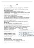
Simple default model predicts everyone at
one of the two options.
Conditional Expectation: The conditional
expectation of Y given X is the average of Y
i.e. Age = 0
with fixing X at a particular value.
The conditional expectation is denoted by Ε ¿
is called a regression function.
Correlation and Causality:
Statistical correlation: X and Y have some systematic relationship.
Cov ( X ,Y )
One measure of correlation: corr ( X , Y ) = ∨corr ( x , y )= √ R2
√ Var X Var (Y )
( )
In order to obtain a measure of explained variance you need to square the correlation
coefficient:
, n
∑ ( x i−x)( y i − y) R =corr ( x , y )=sample corr
2 2 2
i=1
cov ( x , y )=
n−1
Var(X) = Cov(X, X)
Correlation only picks up linear relationships. Correlation is not a causal relationship.
Covariance statistic is not scale free while correlation is.
Under some circumstances, we can interpret correlation as a causal relationship.
Classical Linear Regression Model: We study the conditional expectation E[Y|X] because it
summarises the relationship between Y and X; it may have causal interpretation and it can
be used for forecasting.
We start with: E[Y|X] = α + Xβ α is the intercept and β is the coefficient on X (slope)
E[Y|X] = α + Xβ+ ε , ε=Y −E[Y ∨X ]
By definition E[ε | X ] =0
Terminology: ε regression error, Y dependent/outcome variable, X independent/explanatory
variable/regressor.
Classical Linear Regression Model (CLRM): Data: n observations, (X 1, Y1), …, (Xn, Yn)
Y i=α + X i β +ε i for each i = 1, …, n
1. E [ ε i| X ¿=0 – it basically says E[Yi|Xi] = α + X i β (i.e. this is the conditional expectation)
2. V(ε i| X )=V ( ε i ) =σ
2
This says that the variability of ε i does not depend on Xi. Variance of ε is the same for all i.
3. Cov(ε i , ε j| X )=0 for i≠ j
This says roughly that the information about the ith person has no information about jth
person. Example: survey datasets. Counter example: time series data
2
4. ε i∨X Normal(0 , σ )
The regression error ε has a normal distribution. This is for mathematical convenience
Ordinary Least Squares Estimation (OLS):
Y i=α + β X i +ε i
We want to estimate α , β from the data ( X 1 , Y 1 ) , … ,(X n , Y n)
Idea: We want to make Yi – a – bXi as small as possible
2 2
Least squares estimation: (linear regression): min ( Y 1−a− X 1 b ) + …+ ( Y n −a− X n b )
a ,b
b=¿
Also, a=Y n− X n b
e i=Y i−a− X i b is an estimate of ε i=Y i−α− X i β . We can estimate σ 2=V (ε) by:
n
1
2
sn= ∑
n−2 i=1
2
ei
e i is called regression residual
Inter preting Regression Coefficients:
So, Recap: Y =α + βx + ε :
When X increases by one unit:
Y Log(Y)
X β β∗100 %
When X increases by 1%:
, Y Log(Y)
Log(X) β /100 β%
For ln ( Y ) =a+bx , if b is bigger than 0.1 (growth rate above 10%), then you should be taking
(exp ( b )−1) in order to get the exact % change in Y
For the above case if you do a 4% increase, for example: you do (exp ( 4 b ) −1)
Hypothesis Testing for regression coefficients: We obtain estimates (a, b) for
Y = α + β X 0+ ε
√
n
1
b− β0
∑
n−2 i=1
2
ei
T test: If the null hypothesis is true, T , s^e ( b )= (S.E formula)
s^e (b) n−2 n
∑ ( X i− X n ) 2
i=1
1. Specify the null hypothesis H 0 : β=β 0
2. Alternative hypothesis H1: β ≠ β 0
3. Choose significance level c (e.g. c = 0.05) and find the corresponding values t c/ 2 , t 1−c/2
from the t distribution table
c
[ ]
Ρ T ≤t c = , Ρ T ≥t c =c /2
2
2 1−
2 [ ]
b− β0
4. Compute T = and check whether t c/ 2 ≤ T ≤ t 1−c /2 or T falls outside the interval
s^e (b)
[
tc t c
2
, 1−
2 ]
5. If T is outside the interval, we reject the null. If not, we do not reject the null.
Forecasting: With regression, we can estimate the relationship: Y = α + β X 0+ ε
With estimates (a, b), we want to forecast/predict what the “future” value of Y would be
given X.
1. Choose an appropriate probability level 1 – c
2. Estimate (a, b) from the data and form the predicted value Y^ n +1=a+ X n+1 b
[ ]
2
( X −X n )
^ ( e n+1 ) =s 1+ 1 + n n+ 1
2
V n
3. Compute the variance: n
∑ ( X i − X n )2
i=1
n
1
Where sn= ∑ e 2 , e =Y i−a−b X i
n−2 i=1 i i
2
[
4. Form the confidence interval Y n+1−t c √V ( e n+1 ) , Y n+1 +t 1− c √ V ( e n+1 )
^ ^
2
^ ^
2 ]
Classical linear regression model assumption (CLRM)– normality assumption: ε n+1∨ X N ( 0 , σ 2 )
e n+1 =Y n+1−Y^n+1 = ( α−a ) + ( β−b ) X n+1 +ε n+1
And e n+1 ∨X N ¿
The above procedure is valid under CLRM assumptions. In particular, Cov (ε i , ε j ¿for i≠ j
This CLRM assumption may not be valid in time series models.
Properties of Least Squares (OLS) estimator: Theoretical properties of OLS estimator:
, Unbiasedness: E [ b| X ] =β
This means if we estimate b for multiple datasets, the average of b should be closer to the
true value β
σ2
V [ b|X ] = n
Variance:
∑ ( X i−X n )2
i=1
n ( X i−X n )
ω i=
Linearity: b = ∑ ( X i− X n ) ¿¿ ¿ n
i=1 ∑ ( X j−X n) 2
j=1
It turns out that OLS estimator b has the smallest variance among all the unbiased linear
estimators
OLS estimator is BLUE (Best Linear Unbiased Estimator)
( )
σ2
b∨X Normal β , n
Distribution of b: For hypothesis testing, we used
∑ ( X i−X n ) 2
i=1
n
Also for
∑ e2i 2
or s =
RSS
s= 2
n
i=1
DoF
DoF
( DoF ) s 2n
2
χ 2n−2
σ
Result from mathematical statistics: N(0, 1)/√ χ 2k t k when N(0, 1) and χ 2k are independent
s 2n
b− β0 se ( b )= n
^
where has the distribution Tn-2
s^e (b) ∑ (X i−X n ¿ )2 ¿
i=1
Goodness of Fit:
We defined e i=Y i−Y^ where Yi is what we analyse, Y
^ is a prediction from the regression
model and e i is the residual (error)
n n
1
By taking the average, ∑ ei=Y n−Y^ n∧Y n=Y^n because ∑ ei=0
n i=1 i=1
^ ^
Then Y i−Y n=Y i−Y n+ ei and:
n n n n
2
∑ ( Y i−Y n ) =∑ ( Y^i−Y^n ) +∑ e 2i +2 ∑ ( Y^i−Y^n) ei
2
i=1 i=1 i=1 i =1
TSS = ESS + RSS +0
Total sum of squares (variance of y in the data), explained sum of squares (variance in the of
the predicted part of the regression model), residual sum of squares (variation that we
could not explain using X)
We would like ESS to be larger relative to the RSS as this means that the regression model
explains the data well.
MS = mean sum of squares -> sum of squares/degrees of freedom
Root MSE in a Stata table means mean squares error - √ RSS/ DoF
R squared: measure of goodness of fit:
Voordelen van het kopen van samenvattingen bij Stuvia op een rij:
Verzekerd van kwaliteit door reviews
Stuvia-klanten hebben meer dan 700.000 samenvattingen beoordeeld. Zo weet je zeker dat je de beste documenten koopt!
Snel en makkelijk kopen
Je betaalt supersnel en eenmalig met iDeal, creditcard of Stuvia-tegoed voor de samenvatting. Zonder lidmaatschap.
Focus op de essentie
Samenvattingen worden geschreven voor en door anderen. Daarom zijn de samenvattingen altijd betrouwbaar en actueel. Zo kom je snel tot de kern!
Veelgestelde vragen
Wat krijg ik als ik dit document koop?
Je krijgt een PDF, die direct beschikbaar is na je aankoop. Het gekochte document is altijd, overal en oneindig toegankelijk via je profiel.
Tevredenheidsgarantie: hoe werkt dat?
Onze tevredenheidsgarantie zorgt ervoor dat je altijd een studiedocument vindt dat goed bij je past. Je vult een formulier in en onze klantenservice regelt de rest.
Van wie koop ik deze samenvatting?
Stuvia is een marktplaats, je koop dit document dus niet van ons, maar van verkoper bspurs11. Stuvia faciliteert de betaling aan de verkoper.
Zit ik meteen vast aan een abonnement?
Nee, je koopt alleen deze samenvatting voor €19,10. Je zit daarna nergens aan vast.