100% tevredenheidsgarantie Direct beschikbaar na betaling Zowel online als in PDF Je zit nergens aan vast
logo-home
Cheat Sheet for Data Mining for Business and Governance (880022-M-6) Exam €3,49
In winkelwagen

Overig

Cheat Sheet for Data Mining for Business and Governance (880022-M-6) Exam

2 beoordelingen
 258 keer bekeken  23 keer verkocht

Cheat Sheet with all necessary information to pass the exam of "Data Mining for Business and Governance (-M-6)" at Tilburg University. The course is part of the Master Data Science and Society. It was taught in the academic year 2021/2022 in semester 2, block 3 (January to March 2022) by the lectur...

[Meer zien]
Voorbeeld 1 van de 2  pagina's

  • 21 juni 2022
  • 2
  • 2021/2022
  • Overig
  • Onbekend
Alle documenten voor dit vak (8)

2  beoordelingen

review-writer-avatar

Door: bwsjlsy • 8 maanden geleden

review-writer-avatar

Door: bascrypto • 1 jaar geleden

avatar-seller
hannahgruber
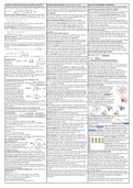
Correlation Coefficient Pearson R for linear correlation, range (-1,1) Supervised Learning: regression: predicting a numeric quantity Supervised Learning: Bagging or Bootstrapping
•Nominator: covariance (to what extent the features change together) •regression analysis describes the relationship between random variables •Train some individual models in parallel to reduce variance of statistical
•Denominator: product of SDs (makes correlations independent of units) •can predict value of one variable based on another variable, show trends learning method. Each model is trained by a random subset of the data.
•output of regression problem = function describing the relation of x and y Supervised Learning: Random Decision Forests (RDFs)
•numerical prediction (for continuous variables) possible ≠ classification •RDFs use bagging as ensemble method, decision tree as individual model
linear regression •randomness is involved through choosing the subsets and features
General Lp-metric “Minkowski-distance”: dist. btw 2 real-valued vectors, •aim: minimize the difference between the predicted and the actual values •RDFs are a way of averaging multiple deep decision trees, trained on
generalization of Euclidean + Manhattan (new parameter “order” / “p“) •measurements: different loss functions or sum of squared errors (sum of different parts of the same training set, goal of reducing the variance
squared difference of predicted vs actual values) •RDFs correct for decision trees' habit of overfitting
Supervised Learning: classification: predicting a class or category •classification tasks: output of RDF is the class selected by most trees
•model to determine most appropriate decision class for a new instance •regression tasks: output = mode of predicted class of the individual trees
2 vectors x = (10, 20, 15, 10, 5) and y = (12, 24, 18, 8, 7), dimensionality •Classifiers draw a decision boundary btw the classes to separate them •complexity of RDFs is determined by number of trees (and their depths)
d = 5 (vectors have five elements), order p = 3 •decision boundaries can be straight / linear or flexible / non-linear •number of trees is a hyperparameter
Euclidean distance (p = 2): dist. btw 2 real-valued vectors, if columns have •the model is learned from the data ‘iterative process’: begins with a •In some DF trees are induced on the same complete set of features
values with differing scales, normalize/standardize numerical values first tentative solution, revises it slightly to see if improves, and repeats this •In random DF trees are induced on randomly selected subsets of features
revision until no more improvement is made, where process is said to have Supervised Learning: Boosting
converged •Training a bunch of individual models in a sequential way. Each individual
Supervised Learning: Logistic regression model learns from mistakes made by the previous model. You train
two vectors x = (10, 20, 15, 10, 5), y = (12, 24, 18, 8, 7), dimensionality d = 5 • regression model used for classification in combination with a threshold predictors sequentially, each time trying to correct the predecessor
Manhattan distance (p = 1): dist. between two real-valued vectors, useful •regression model when the dependent variable is categorical (misclassification of data points). Each tree is fit on a modified version of
to vectors that describe objects on a uniform grid, i.e., two vectors in an •the output function is a sigmoid / logit curve (logarithmic) the original dataset.
integer feature space •possible to use polynomial functions to fit a complex decision boundary no bagging, converts several weak learners to 1 strong, ↓ bias, (variance)
k-nn (k nearest neighbor) → find k nearest neighbor for each data point Supervised Learning: Ada Boost (adaptive boosting algorithm)
vectors x = (10, 20, 15, 10, 5) and y = (12, 24, 18, 8, 7), dimensionality d = 5 •mainly used in classification, but can also be used in regression • boosting ensemble model that works especially well with decision tree
Categorical attributes (Hamming distance): distance between two binary •simple idea: similarity = we look for the most similar exp in the training set •learns from the previous mistakes by increasing the weight of
vectors •measure similarity by calculating the distance (see distance functions) misclassified data points (focusing on them due to higher weight)
•Given a test point, measure the distances to all the training points, and •the second classifier is then trained on the updated weights and so on
pick k nearest ones. Their labels define estimated label of the test point •disadv to bagging: technique cannot be parallelized, doesn’t scale well
•the larger the data set, the more time is required to calculate all distances Supervised Learning: Naïve Bayes Classifier
•k-nn is a lazy learner: it doesn't learn a model from the training data but •fast, easy implement but predic. must be independent (wrong in real life)
𝐿𝑖𝑘𝑒𝑙𝑖ℎ𝑜𝑜𝑑∗𝑃𝑟𝑖𝑜𝑟
“memorizes” the training dataset, memorization = learning-as- Bayes’ rule 𝑃𝑜𝑠𝑡𝑒𝑟𝑖𝑜𝑟 = 𝑀𝑎𝑟𝑔𝑖𝑛𝑎𝑙𝑖𝑧𝑎𝑡𝑖𝑜𝑛
vectors x = (0, 0, 0, 0, 0, 1) and y = (0, 0, 0, 0, 1, 0), dimensionality d = 6 memorization (most basic form of learning), lazy learning methods simply 𝑃(𝐵 |𝐴)∗𝑃(𝐴)
store the (training) data and generalizing beyond these data is postponed •𝑃(𝐴|𝐵) = 𝑃(𝐵)
=
Similarity Function until an explicit request is made (until receiving test data), generalization 𝑃𝑟𝑜𝑑𝑢𝑐𝑡 𝑜𝑓 𝑝𝑟𝑜𝑏𝑠 𝑎𝑙𝑜𝑛𝑔 𝑡ℎ𝑒 𝑏𝑟𝑎𝑛𝑐ℎ 𝑡ℎ𝑟𝑜𝑢𝑔ℎ 𝐴 𝑡𝑒𝑟𝑚𝑖𝑛𝑡𝑖𝑛𝑔 𝑎𝑡 𝐷
•Correlation of the training data is delayed, opposite: eager learner (e.g., decision tree) 𝑆𝑢𝑚 𝑜𝑓 𝑝𝑟𝑜𝑑𝑢𝑐𝑡𝑠 𝑜𝑓 𝑡ℎ𝑒 𝑝𝑟𝑜𝑏𝑠 𝑎𝑙𝑜𝑛𝑔 𝑒𝑎𝑐ℎ 𝑏𝑟𝑎𝑛𝑐ℎ 𝑡𝑒𝑟𝑚𝑖𝑛𝑎𝑡𝑖𝑛𝑔 𝑎𝑡 𝐷
coefficient: •Posterior: The prob of “A” being true given “B” is True
starts classifying when it receives training data. it takes long time learning
range [-1,+1] and less time classifying data •Likelihood: The prob of “B” being true, given “A” is true (has been true)
•Cosine similarity relates to the angle between different vectors •role of k: k defines how many neighbors are checked; as k gets larger, •Prior: The prob of “A” being true. This is known, has happened already
•similar scores: score vectors in same direction, angle between them is decision boundaries get smoother, risk of underfitting for high k because •Marginalization: The probability of “B” being True
near 0 deg., cosine of angle is near 1 i.e., 100% data is less correctly labeled, risk of overfitting for small k since labeling is •Given dataset with 2 classes (Dem,Rep) and 3 features (A,B,C):
•unrelated scores: score vectors are nearly orthogonal, angle between defined too much by the training data •P(Dem|data) = P(A|Dem) x P(B|Dem) x P(C|Dem) x P(Dem) / P(A, B, C)
them is near 90 deg., cosine of angle is near 0 i.e., 0% •weight features: some dimensions may be more informative for defining •P(Rep|data) = P(A|Rep) x P(B|Rep) x P(C|Rep) x P(Rep) / P(A, B, C)
•opposite scores: score vectors in opposite direction, angle between them the class than others, attach a larger weight to that dimension, give •IF P(Dem|data) > P(Rep|data) THEN class is Dem ELSE class is Rep
is near 180 deg., cosine of angle is near -1 i.e., -100% different weights to different data points to alter their influence Supervised Learning: Support Vector Machines a.k.a. Kernel Machines
•hyperparameters: k, neighbor weights, distance metric •simplest model: Linear SVM places a straight line between the classes
Evaluating Model Performance: Metrics for Regression Tasks •when k is increasing the model boundaries get smoother and smoother: •like logistic regression, but “optimal”
•Coefficient of determination (R2): k = 1 → model is overfitting (every datapoint is assigned to its own class) •SVM produce better dec. boundaries with larger distances in-between
measures how well model f predicts k = 17 → model is underfitting •using kernels, SVMs make more complex dec. boundaries than with lines
targets relative to the mean, •train and test error as a function of k to decide on hyperparameters: check Supervised Learning: Kernel
Equivalent to proportion of error rate for different values of k, performance on training and test set •kernel performs a mathematical operation on
variance explained by f should be similar (intersection in graph) instances in two classes that are not linearly
•Mean Absolute Error (MAE), Root •advantages of k-nn: fast learner, fast classification possible (using smart separable, so that they do become linearly
Mean Squared Error (RMSE) and indexing structures like k-d-trees), directly provides illustrative examples separable. (e.g., in a higher dimension)
Mean Squared Error (MSE): Errors Supervised Learning: Decision Tree Classifier (e.g., Dichotomiser 3 “ID3”) •Radial Basis Function has 2 hyperparameter:
describe the difference between •decision / internal nodes test for a specific attribute, branches are the c is proportional to the misclassification
true value y and predicted value outcome of tests, leaf nodes represent classification or decision, root node penalty (relates to error): lower c means low
•Root Mean Squared Error (RMSE): is the topmost decision node error; higher c means higher error)
RMSE includes the squared term so •test a binary condition on one feature at a time, result is a decision gamma is the rang of influence in feature space
outliers will affect the distance much more than when using MAE, RMSE is boundary (collection of lines (perpendicular to the feature axes) to cluster (sigma = 1 / gamma): when gamma becomes
equal to Mean Square Error (MSE) when not taking the root the data) larger, the model becomes more complex and
•Mean Absolute Error (MAE): depends on distances between predicted and •Basic Algorithm: Initially, all (training) instances are assigned to the root. closer around the single data points
actual values The next attribute (test) is selected – splitting strategy. The training set is
Evaluating Model Performance: Metrics for Classification Tasks partitioned using the split attribute. Proceed for all partitions recursively
•we want to know if there is a dominant / overrepresented class (this one (locally optimizing algorithm)
will be predicted more often because it is more present) •Stopping criterion: No more splitting attributes or all instances of a node
•Confusion Matrix belong to exactly one class (data cannot be split further)
(unbalanced classes in •splitting strategy: Use quality function to determine goodness of them (in- Cross Validation (out-of-sample testing): how the results of a statistical
the confusion matrix will formation gain, information gain ratio, gini index)
lead to diff. results for analysis will generalize to an independent data set
•entropy to measure the amount of information Hold out method: Separate into training set
the single metrics) attached to each attribute (measure of disorder, purity), pure node: E=0, (used for training) and testing set (the rest
•Type I error: false positive, Type II error: false negative maximal impurity (50/50): E=max
•accuracy compares the true prediction vs the whole set of datapoints of the data), train the model on training set,
E(outlook sunny)=E(sunny yes(2)/total sunny(5), sunny no(3)/total sunny(5 calculate accuracy
(TP + TN) / (TP + FN + FP + TN) E(outlook sunny)= [-(2/5) * log2 (2/5)] + [-(3/5) * log2 (3/5)] = 0.971
•precision is the hit-rate (true positives vs the ones predicted as positives) do this for all possible outcomes of outlook (sunny, overcast, rainy) K-fold cross validation: Split randomly into k
(TP) / (TP + FP) subsets. Use 1 as testing set to evaluate a
•entropy weighted sum per subset / feature (=outlook) model generated by using others as training
•recall / sensitivity is the true positive rate (true positives vs the actual E(v in outlook)=E(sunny)*(sunny/outlook)+…+E(rainy)*(rainy/outlook)
positives) sets. Repeat this with all subsets, average
5x sunny, 5x overcast, 5x rainy, 14 in total times their entropy errors. Nice for small datasets bc all data is used for training + testing. If
(TP) / (TP + FN) or (TP) / diseased (5/14) * 0.971 + (4/14) * 0 + (5/14) * 0.971 = 0.693 hyperpara. is included, separate test set at the start, then split remaining
•specificity: (TN) / (TN + FP) or (TN) / healthy •information gain per feature (=outlook), compare the single features data in training and validation sets and iterate over all combinations
•F / F1 score combines precision + recall, result is kind of mean of the two gain(outlook)=E(9,5) – weighted sum(outlook) → 0.94 − 0.693 = 0.247
Nested cross validation: Like k-fold vali., but
2* [ Precision * Recall ] / [ Precision + Recall ] E(9, 5) because 9x yes and 5x no, 14 observations in this feature in total: also iterate over the “outer loop” of the test
Area Under ROC (receiver operating [-(9/14) * log2 (9/14)] + [-(5/14) * log2 (5/14)] = 0.94 data additionally to the “inner loop” of
characteristics) Curve •Complexity of induced model = tree depth (num of decision boundaries) validation and training data.
•measure between 0.5 and 1.0, the closer •The information gain measure is biased towards choosing attributes with Leave-one-out: Use one of examples to test a
the value to 1.0 the more accurate the many values (extreme case: ID numbers) which may result in overfitting. model generated by using the other exp.
model can distinguish between the •gain ratio considers number and size of branches to avoid overfitting Calculate judgement for this model: 0 if
classes, can inspect outcome for different •use pruning to reduce complexity of the final classifier and to improve model and exp are consistent, 1, otherwise.
thresholds (criterion) predictive accuracy by reduction of overfitting Repeat these 2 steps for all exp & average the obtained judgement values.
Overfitting, Underfitting if M fits, low error on both, train, test data •two types / procedures: pre- and post-pruning which are differentiated Hyperparameters and Model Parameters
Overfitting: M is too complex for the data, low error train, high error test based on their approach in the tree (top-down or bottom-up) •Hyperparameters aren’t set during learning on training data but must be
Underfitting: M is too simple for the data, high error train, high error test
•pre-pruning: stop criterion to stops growing the tree when the condition is defined by the programmer and tuned on validation set
Bias-Variance Tradeoff: conflict trying to simultaneously minimize the two
met (e.g., statistically significant association between attribute and class, •Model Parameter “learnt”: Required by the model when making
sources of error prevent supervised learning algorithms from generalizing:
max. tree depth or information gain (Attr)> minGain), problem: induction predictions. Values define the ‘skill’ of the model on your problem. Are
•bias error: error from wrong assumptions in the learning algorithm. High of algorithm might stop too early
learned from data. Not set manually by the practitioner. Often saved as
bias can cause an algorithm to miss the relevant relations between
•post-pruning: after the construction process has been finished, replace part of the learned model. E.g., coefficient in a linear/logistic regression.
features and target outputs (underfitting).
nodes and subtrees with leaves to reduce complexity •Model Hyperparameters “chosen”: Often used in processes to help
•variance: error from sensitivity to small fluctuations in the training set.
•bottom-up pruning: starts at the last node / lowest point of tree, checks estimate model parameters. Not learned during the training purpose but
High variance may result from an algorithm modeling the random noise in
the relevance of each individual node, if not relevant drop node/replace it chosen actively. Can be set using heuristics. Often specified by the
the training data (overfitting).
by a leaf practitioner. Often tuned for a given predictive modeling problem. E.g., K
Supervised Learning: Stratification/Splitting Data: similar characteristics
•top-down pruning: starts at the root, checks if the node is relevant for the in K-nearest neighbors
Model selection
classification of all n items, if not removes the node and its entire sub-tree Supervised Learning: Grid Search to find best hyperparameter settings
1. Define feature sets
•Advantages of decision trees: simple to understand & interpret, can work •Systematic search, computationally expensive: Manually choose values to
2. Choose hyperparameters: Choose range of values to check
with relatively little data, help find which feature is most important for test for each hyperparameter combination, check validation
3. Check performance on train and validation data: For as many
classification accuracy/error for all of them
combinations of the above as you can afford
4. Pick combination with lowest error • Grid Layout: structured values, Random Layout: randomly choose sets of
5. Test it on the test set to check if it generalizes well hyperparameter and decide for the one that performs the best

Voordelen van het kopen van samenvattingen bij Stuvia op een rij:

Verzekerd van kwaliteit door reviews

Verzekerd van kwaliteit door reviews

Stuvia-klanten hebben meer dan 700.000 samenvattingen beoordeeld. Zo weet je zeker dat je de beste documenten koopt!

Snel en makkelijk kopen

Snel en makkelijk kopen

Je betaalt supersnel en eenmalig met iDeal, creditcard of Stuvia-tegoed voor de samenvatting. Zonder lidmaatschap.

Focus op de essentie

Focus op de essentie

Samenvattingen worden geschreven voor en door anderen. Daarom zijn de samenvattingen altijd betrouwbaar en actueel. Zo kom je snel tot de kern!

Veelgestelde vragen

Wat krijg ik als ik dit document koop?

Je krijgt een PDF, die direct beschikbaar is na je aankoop. Het gekochte document is altijd, overal en oneindig toegankelijk via je profiel.

Tevredenheidsgarantie: hoe werkt dat?

Onze tevredenheidsgarantie zorgt ervoor dat je altijd een studiedocument vindt dat goed bij je past. Je vult een formulier in en onze klantenservice regelt de rest.

Van wie koop ik deze samenvatting?

Stuvia is een marktplaats, je koop dit document dus niet van ons, maar van verkoper hannahgruber. Stuvia faciliteert de betaling aan de verkoper.

Zit ik meteen vast aan een abonnement?

Nee, je koopt alleen deze samenvatting voor €3,49. Je zit daarna nergens aan vast.

Is Stuvia te vertrouwen?

4,6 sterren op Google & Trustpilot (+1000 reviews)

Afgelopen 30 dagen zijn er 53340 samenvattingen verkocht

Opgericht in 2010, al 14 jaar dé plek om samenvattingen te kopen

Start met verkopen
€3,49  23x  verkocht
  • (2)
In winkelwagen
Toegevoegd